A Guide to Scientific Computing with Open Source Tools

Historically, computational science has largely been confined to the realm of research scientists and doctoral candidates. However, over the years – perhaps unbeknownst to the larger software community – us scientific computing eggheads have been quietly compiling collaborative open-source libraries that handle the vast majority of the heavy lifting. The result is that it is now easier than ever to implement mathematical models, and while the field may not yet be ready for mass-consumption, the bar to successful implementation has been drastically lowered. Developing a new computational codebase from scratch is a huge undertaking, measured typically in years, but these open source scientific computing projects are making it possible to run with accessible examples to relatively quickly leverage these computational abilities.

Since the purpose of scientific computing is to provide scientific insight into real systems that exist in nature, the discipline represents the cutting edge in making computer software approach reality. In order to make software that mimics the real world to a very high degree of both accuracy and resolution, complex differential mathematics must be invoked, requiring knowledge that is rarely found beyond the walls of universities, national labs, or corporate R&D departments. On top of this, significant numerical challenges present themselves when attempting to describe the continuous, infinitesimal fabric of the real world using the discrete language of zeros and ones. An exhaustive effort of careful numerical transformation is necessary to render algorithms that are both computationally tractable, and which render meaningful results. In other words, scientific-computing is heavy duty.

Open Source Tools for Scientific Computing

I personally am particularly fond of the FEniCS project, using it for my thesis work, and will demonstrate my bias in selecting that for our code example for this tutorial. (There are other very high quality projects such as DUNE which one could use as well.)

FEniCS is self-described as “a collaborative project for the development of innovative concepts and tools for automated scientific computing, with a particular focus on automated solution of differential equations by finite element methods.” This is a powerful library for solving a huge array of problems and scientific computing applications. Its contributors include Simula Research Laboratory, the University of Cambridge, the University of Chicago, Baylor University, and KTH Royal Institute of Technology, who have collectively built it into an invaluable resource over the course of the last decade (see the FEniCS codeswarm).

What is rather astonishing is just how much effort the FEniCS library has shielded us from. To get a sense of the amazing depth and breadth of the topics the project covers one can view their open source text book, where Chapter 21 even compares various finite element schemes for solving incompressible flows.

Behind the scenes the project has integrated for us a large set of open source scientific computing libraries, which may be of interest or of use directly. These include, in no particular order, the projects which the FEniCS project calls out:

• PETSc: A suite of data structures and routines for the scalable (parallel) solution of scientific applications modeled by partial differential equations.
• Trilinos Project: A set of robust algorithms and technologies for solving both linear and non-linear equations, developed from work at Sandia National Labs.
• uBLAS: “A C++ template class library that provides BLAS level 1, 2, 3 functionality for dense, packed and sparse matrices and many numerical algorithms for linear algebra.”
• GMP: A free library for arbitrary precision arithmetic, operating on signed integers, rational numbers, and floating-point numbers.
• UMFPACK: A set of routines for solving unsymmetric sparse linear systems, Ax=b, using the Unsymmetric MultiFrontal method.
• ParMETIS: An MPI-based parallel library that implements a variety of algorithms for partitioning unstructured graphs, meshes, and for computing fill-reducing orderings of sparse matrices.
• NumPy: The fundamental package for scientific computing with Python.
• CGAL: Efficient and reliable geometric algorithms in the form of a C++ library.
• SCOTCH: A software package and libraries for sequential and parallel graph partitioning, static mapping and clustering, sequential mesh and hypergraph partitioning, and sequential and parallel sparse matrix block ordering.
• MPI: A standardized and portable message-passing system designed by a group of researchers from academia and industry to function on a wide variety of parallel computers.
• VTK: An open-source, freely available software system for 3D computer graphics, image processing and visualization.
• SLEPc: A software library for the solution of large scale sparse eigenvalue problems on parallel computers.

This list of external packages integrated into the project gives us a sense of its inherited capabilities. For example, having integrated support for MPI allows for scaling across remote workers in a compute cluster environment (i.e., this code will run on a super computer or your laptop).

It is also interesting to note that there are many applications beyond scientific computing for which these projects could be utilized, including financial modeling, image processing, optimization problems, and perhaps even video games. It would be possible, for example, to create a video game which uses some of these open source algorithms and techniques to solve for a two dimensional fluid flowing, such as that of ocean/river currents which a player would interact with (perhaps try and sail a boat across with varying wind and water flows).

A Sample Application: Leveraging Open Source for Scientific Computing

Here I will try to give a flavor for what developing a numerical model involves by showing how a basic Computational Fluid Dynamics scheme is developed and implemented in one of these open source libraries - in this case the FEniCS project. FEnICS provides APIs in both Python and C++. For this example, we’ll be using their Python API.

We will discuss some rather technical content, but the goal will simply be to give a taste of what developing such scientific computing code entails, and just how much legwork today’s open source tools do for us. In the process, hopefully we will help demystify the complex world of scientific computing. (Note that an Appendix is provided that details all the mathematical and scientific underpinnings for those who are interested in that level of detail.)

DISCLAIMER: For those readers with little or no background in scientific computing software and applications, parts of this example may make you feel like this:

If so, don’t despair. The main takeaway here is the extent to which existing open source projects can greatly simplify many of these tasks.

With that in mind, let’s begin by looking at the FEnICS demo for incompressible Navier-Stokes. This demo models pressure and velocity of an incompressible fluid flowing through an L-shaped bend, such as a plumbing pipe.

The description on the demo page linked gives an excellent, concise setup of the necessary steps for running the code, and I encourage you to take a quick look to see what is involved. To summarize, the demo will solve the velocity and pressure through the bend for the incompressible flow equations. The demo runs a short simulation of the fluid flowing over time, animating the results as it goes. This is accomplished by setting up the mesh representing the space in the pipe, and using the Finite Element Method to numerically solve the velocity and pressure at each point on the mesh. We then iterate through time, updating the velocity and pressure fields as we go, again using the equations we have at our disposal.

The demo works well as-is, but we are going to modify it slightly. The demo uses the Chorin split, but we are going to use the slightly different method inspired by Kim and Moin instead, which we hope is more stable. This just requires us to change the equation used to approximate the convective and viscous terms, but to do so we need to store the velocity field of the the previous time step, and add two additional terms to the update equation, which will use that previous information for a more accurate numerical approximation.

So let’s make this change. First, we add a new Function object to the setup. This is an object that represents an abstract mathematical function such as a vector or scalar field. We’ll call it un1 it will store the previous velocity field

on our function space V.

...
# Create functions	(three distinct vector fields and a scalar field)
un1 = Function(V)	# the previous time step's velocity field we are adding
u0 = Function(V)	# the current velocity field
u1 = Function(V)	# the next velocity field (what's being solved for)
p1 = Function(Q)	# the next pressure field (what's being solved for)
...

Next, we need to change the way the “tentative velocity” is updated during each step of the simulation. This field represents the approximated velocity at the next time step when pressure is ignored (at this point pressure is not yet known). This is where we replace the Chorin split method with the more recent Kim and Moin fractional step method. In other words, we will change the expression for the field F1:

Replace:

# Tentative velocity field (a first prediction of what the next velocity field is)
# for the Chorin style split
# F1 = change in the velocity field +
#      convective term +
#      diffusive term -
#      body force term

F1 = (1/k)*inner(u - u0, v)*dx + \
     inner(grad(u0)*u0, v)*dx + \
     nu*inner(grad(u), grad(v))*dx - \
     inner(f, v)*dx

With:

# Tentative velocity field (a first prediction of what the next velocity field is)
# for the Kim and Moin style split
# F1 = change in the velocity field +
#      convective term +
#      diffusive term -
#      body force term

F1 = (1/k)*inner(u - u0, v)*dx + \ 
     (3.0/2.0) * inner(grad(u0)*u0, v)*dx - (1.0/2.0) * inner(grad(un1)*un1, v)*dx + \ 
     (nu/2.0)*inner(grad(u+u0), grad(v))*dx - \ 
     inner(f, v)*dx 

so that the demo now uses our updated method for solving for the intermediate velocity field when it uses F1.

Finally, make sure we are updating the previous velocity field, un1, at the end of each iteration step

...
# Move to next time step
un1.assign(u0)		# copy the current velocity field into the previous velocity field
u0.assign(u1)		# copy the next velocity field into the current velocity field
...

So that the following is the complete code from our FEniCS CFD demo, with our changes included:

"""This demo program solves the incompressible Navier-Stokes equations
on an L-shaped domain using Kim and Moin's fractional step method."""

# Begin demo

from dolfin import *

# Print log messages only from the root process in parallel
parameters["std_out_all_processes"] = False;

# Load mesh from file
mesh = Mesh("lshape.xml.gz")

# Define function spaces (P2-P1)
V = VectorFunctionSpace(mesh, "Lagrange", 2)
Q = FunctionSpace(mesh, "Lagrange", 1)

# Define trial and test functions
u = TrialFunction(V)
p = TrialFunction(Q)
v = TestFunction(V)
q = TestFunction(Q)

# Set parameter values
dt = 0.01
T = 3
nu = 0.01

# Define time-dependent pressure boundary condition
p_in = Expression("sin(3.0*t)", t=0.0)

# Define boundary conditions
noslip  = DirichletBC(V, (0, 0),
                      "on_boundary && \
                       (x[0] < DOLFIN_EPS | x[1] < DOLFIN_EPS | \
                       (x[0] > 0.5 - DOLFIN_EPS && x[1] > 0.5 - DOLFIN_EPS))")
inflow  = DirichletBC(Q, p_in, "x[1] > 1.0 - DOLFIN_EPS")
outflow = DirichletBC(Q, 0, "x[0] > 1.0 - DOLFIN_EPS")
bcu = [noslip]
bcp = [inflow, outflow]

# Create functions
un1 = Function(V)
u0 = Function(V)
u1 = Function(V)
p1 = Function(Q)

# Define coefficients
k = Constant(dt)
f = Constant((0, 0))

# Tentative velocity field (a first prediction of what the next velocity field is)
# for the Kim and Moin style split
# F1 = change in the velocity field +
#     convective term +
#     diffusive term -
#     body force term

F1 = (1/k)*inner(u - u0, v)*dx + \
     (3.0/2.0) * inner(grad(u0)*u0, v)*dx - (1.0/2.0) * inner(grad(un1)*un1, v)*dx + \
     (nu/2.0)*inner(grad(u+u0), grad(v))*dx - \
     inner(f, v)*dx 
a1 = lhs(F1)
L1 = rhs(F1)

# Pressure update
a2 = inner(grad(p), grad(q))*dx
L2 = -(1/k)*div(u1)*q*dx

# Velocity update
a3 = inner(u, v)*dx
L3 = inner(u1, v)*dx - k*inner(grad(p1), v)*dx

# Assemble matrices
A1 = assemble(a1)
A2 = assemble(a2)
A3 = assemble(a3)

# Use amg preconditioner if available
prec = "amg" if has_krylov_solver_preconditioner("amg") else "default"

# Create files for storing solution
ufile = File("results/velocity.pvd")
pfile = File("results/pressure.pvd")

# Time-stepping
t = dt
while t < T + DOLFIN_EPS:

    # Update pressure boundary condition
    p_in.t = t

    # Compute tentative velocity step
    begin("Computing tentative velocity")
    b1 = assemble(L1)
    [bc.apply(A1, b1) for bc in bcu]
    solve(A1, u1.vector(), b1, "gmres", "default")
    end()

    # Pressure correction
    begin("Computing pressure correction")
    b2 = assemble(L2)
    [bc.apply(A2, b2) for bc in bcp]
    solve(A2, p1.vector(), b2, "cg", prec)
    end()

    # Velocity correction
    begin("Computing velocity correction")
    b3 = assemble(L3)
    [bc.apply(A3, b3) for bc in bcu]
    solve(A3, u1.vector(), b3, "gmres", "default")
    end()

    # Plot solution
    plot(p1, title="Pressure", rescale=True)
    plot(u1, title="Velocity", rescale=True)

    # Save to file
    ufile << u1
    pfile << p1

    # Move to next time step
    un1.assign(u0)
    u0.assign(u1)
    t += dt
    print "t =", t

# Hold plot
interactive()

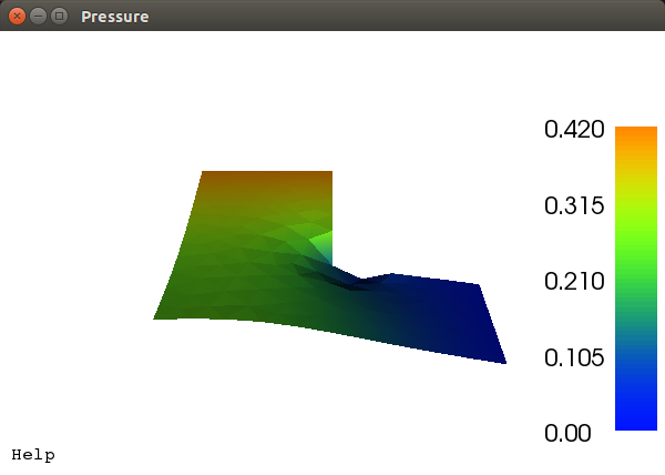
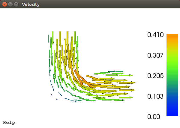
Running the program shows the flow around the elbow. Run the scientific computing code yourself to see it animate! Screens of the final frame are presented below.

Relative pressures in the bend at the end of the simulation, scaled and colored by magnitude (non-dimensional values):

Relative velocities in the bend at the end of the simulation as vector glyphs scaled and colored by magnitude (non-dimensional values).

So what we have done is taken an existing demo, which happens to implement a scheme very similar to ours rather easily, and modified it to use better approximations by using information from the previous time step.

At this point you might be thinking that was a trivial edit. It was, and that is largely the point. This open source scientific computing project has allowed us to quickly implement a modified numerical model by changing four lines of code. Such changes may take months in large research codes.

The project has many other demos which could be used as a starting point. There are even a number of open source applications built on the project which implement various models.

Conclusion

Scientific computing and its applications are indeed complex. There’s no getting around that. But as is increasingly true in so many domains, the ever-growing landscape of available open source tools and projects can significantly simplify what would otherwise be extremely complicated and tedious programming tasks. And perhaps the time is even near where scientific computing becomes accessible enough to find itself being readily utilized beyond the research community.

---

APPENDIX: Scientific and Mathematical Underpinnings

For those interested, here are the technical underpinnings of our Computational Fluid Dynamics guide above. What follows will serve as a very useful and concise summary of topics that are typically covered over the course of a dozen or so graduate level courses. Graduate students and mathematical types interested in a deep understanding of the topic may find this material quite engaging.

Fluid Mechanics

“Modeling,” in general, is the process of solving some real system with a series approximations. The model, will often involve continuous equations ill-suited for computer implementation, and so must be further approximated with numerical methods.

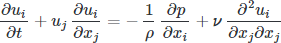
For fluid mechanics, let’s start this guide from the fundamental equations, the Navier-Stokes equations, and use that to develop a CFD scheme.

The Navier-Stokes equations are a series of partial differential equations (PDEs) which describe fluid flows very well and are thus our starting point. They can be derived from mass, momentum, and energy conservation laws thrown through a Reynolds Transport Theorem and applying Gauss’s theorem and invoking Stoke’s Hypothesis. The equations require a continuum assumption, where it is assumed we have enough fluid particles to give statistical properties such as temperature, density and velocity meaning. In addition a linear relationship between the surface stress tensor and strain rate tensor, symmetry in the stress tensor, and isotropic fluid assumptions are needed. It is important to know the assumptions we make and inherit during this development so that we can evaluate the applicability in the resulting code. The Navier-Stokes equations in Einstein notation, without further ado:

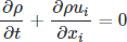
Conservation of mass:

Conservation of momentum:

Conservation of energy:

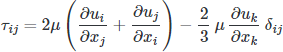
where the deviatoric stress is:

While very general, governing most fluid flows in the physical world, they are not of much use directly. There are relatively few known exact solutions to the equations, and a $1,000,000 Millennium Prize is out there for anyone who can solve the existence and smoothness problem. The important part is we have a starting point for the development of our model by making a series of assumptions to reduce the complexity (they are some of the hardest equations in classical physics).

To keep things “simple” we will use our domain specific knowledge to make an incompressible assumption on the fluid, and assume constant temperatures such that the conservation of energy equation, which becomes the heat equation, is not needed (decoupled). We now have two equations, still PDEs, but significantly simpler while still resolving a large number of real fluid problems.

Continuity equation

Momentum equations

At this point we now have a nice mathematical model for incompressible fluid flows (low speed gasses and liquids such as water, for example). Solving these equations directly by hand is not easy, but it is nice in that we can obtain “exact” solutions for simple problems. Using these equations to address problems of interest, say air flowing over a wing, or water flowing through some system, requires that we solve these equations numerically.

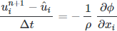
Building a Numerical Scheme

In order to solve more complex problems using the computer, a method to numerically solve our incompressible equations is needed. Solving partial differential equations, or even differential equations, numerically is not trivial. However, our equations in this guide have a particular challenge (surprise!). That is, we need to solve the momentum equations while keeping the solution divergence free, as required by continuity. A simple time integration through something like Runge-Kutta method is made difficult since the continuity equation does not have a time derivative within it.

There is no correct, or even best, method for solving the equations, but there are many workable options. Over the decades several approaches have been found to address the issue, such as reformulating in terms of vorticity and the stream-function, introducing artificial compressibility, and operator splitting. Chorin (1969), and then Kim and Moin (1984, 1990), formulated a very successful and popular fractional step method which will allow us to integrate the equations while solving for the pressure field directly, rather then implicitly. The fractional step method is a general method for approximating equations by splitting their operators, in this case splitting along pressure. The approach is relatively simple and yet robust, motivating its choice here.

First, we need to numerically discritize the equations in time so that we may step from one point in time to the next. In following Kim and Moin (1984), we will use the second-order-explicit Adams-Bashforth method for the convective terms, the second-order-implicit Crank-Nicholson method for the viscous terms, a simple finite difference for the time derivative, while neglecting the pressure gradient. These choices are by no means the only approximations that can be made: their selection is part of the art in building the scheme by controlling the numerical behavior of the scheme.

The intermediate velocity can now be integrated, however, it ignores the contribution of pressure and is now divergent (incompressibility requires it to be divergent free). The remainder of the operator is needed to bring us to the next time step.

where

is some scalar we need to find which results in a divergent free velocity. We can find by taking the divergence of the correction step,

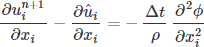
where the first term is zero as required by continuity, yielding a Poisson equation for a scalar field which will provide a solenoidal (divergent free) velocity at the next time step.

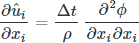
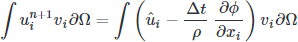
As Kim and Moin (1984) show,

is not exactly the pressure as a result of the operator splitting, but it can be found by

.

At this point in the tutorial we are doing rather well, we have temporally discritized the governing equations so that we may integrate them. We now need to spatially discritize the operators. A number of methods exist with which we could accomplish this, the Finite Element Method, the Finite Volume Method, and the Finite Difference Method, for example. In Kim and Moin’s (1984) original work, they proceed with the Finite Difference Method. The method is advantagous for its relative simplicity and computational efficiency, but suffers for complex geometries as it requires a structured mesh.

The Finite Element Method (FEM) is a convenient selection for its generality and has some very nice open source projects aiding in its use. In particular it handles real geometries in one, two and three dimensions, scales for very large problems on machine clusters, and is relatively easy to use for high order elements. Typically the method is the slower of the three, however it will give us the most mileage across problems, so we will use it here.

Even when implementing the FEM there are many choices. Here we will use the Galerkin FEM. In doing so, we cast the equations in weighted residual form by multiply each by a test function

for the vectors and for the scalar field, and integrating over the domain . We then perform partial integration on any high order derivatives using Stoke’s theorem or the Divergence theorem. We then pose the variational problem, yielding our desired CFD scheme.

We now have a nice mathematical scheme in a “convenient” form for implementation, hopefully with some sense of what was needed to get there (lots of math, and methods from brilliant researchers that we pretty much copy and tweak).