From Solving Equations to Deep Learning: A TensorFlow Python Tutorial

There have been some remarkable developments lately in the world of artificial intelligence, from much publicized progress with self-driving cars to machines now composing Chopin imitations or just being really good at video games.

Central to these advances are a number of tools around to help derive deep learning and other machine learning models, with Torch, Caffe, and Theano amongst those at the fore. However, since Google Brain went open source in November 2015 with their own framework, TensorFlow, we have seen the popularity of this software library skyrocket to be the most popular deep learning framework.

Why has this happened? Reasons include the wealth of support and documentation available, its production readiness, the ease of distributing calculations across a range of devices, and an excellent visualization tool: TensorBoard.

Ultimately, TensorFlow manages to combine a comprehensive and flexible set of technical features with great ease of use.

In this article, you will gain an understanding of the mechanics of this tool by using it to solve a general numerical problem, quite outside of what machine learning usually involves, before introducing its uses in deep learning with a simple neural network implementation.

Before You Begin

A basic knowledge of machine learning methods is assumed. If you need catching up, check out this very useful post.

As we will be demonstrating the Python API, an understanding of Numpy is also beneficial.

To set up TensorFlow, please follow the instructions found here.

If you are using Windows, it should be noted that, at the time of writing, you must use Python 3.4+, not 2.7.

Then when you are ready, you should be able to import the library with:

import tensorflow as tf

Step 1 of 2 to a TensorFlow Solution: Create a Graph

The construction of TensorFlow programs generally consist of two major steps, the first of which is to build a computational graph, which will describe the computations you wish to carry out, but not actually carry them out or hold any values.

As with any graph, we have nodes and edges. The edges represent tensors, a tensor representing an n-dimensional array. For example, a tensor with dimension (or rank in TensorFlow speak) 0 is a scalar, rank 1 a vector, rank 2 a matrix and so on.

Nodes represent operations which produce an output tensor, taking tensors as inputs if needed. Such operations include additions (tf.add), matrix multiplications (tf.matmul), and also the creation of constants (tf.constant).

So, let’s combine a few of these for our first graph.

a = tf.constant([2.5, 2])
b = tf.constant([3, 6], dtype=tf.float32)
total = tf.add(a, b)

Here we have created three operations, two of them to create constant 1-d arrays.

The data types are inferred from the values argument passed in, or you can denote these with the dtype argument. If I hadn’t have done this for b, then an int32 would have been inferred and an error thrown as tf.add would have been trying to define an addition on two different types.

Step 2 of 2 to a TensorFlow Solution: Execute the Operations

The graph is defined, but in order to actually do any calculations on it (or any part of it) we have to set up a TensorFlow Session.

sess = tf.Session()

Alternatively, if we are running a session in an interactive shell, such as IPython, then we use:

sess = tf.InteractiveSession()

The run method on the session object is one way to evaluate a Tensor.

Therefore, to evaluate the addition calculation defined above, we pass ‘total’, the Tensor to retrieve, which represents the output of the tf.add op.

print(sess.run(total)) # [ 5.5  8. ]

At this point, we introduce TensorFlow’s Variable class. Whereas constants are a fixed part of the graph definition, variables can be updated. The class constructor requires an initial value, but even then, variables need an operation to explicitly initialize them before any other operations on them are carried out.

Variables hold the state of the graph in a particular session so we should observe what happens with multiple sessions using the same graph to better understand variables.

# Create a variable with an initial value of 1
some_var = tf.Variable(1)

# Create op to run variable initializers
init_op = tf.global_variables_initializer()
 
# Create an op to replace the value held by some_var to 3
assign_op = some_var.assign(3)
 
# Set up two instances of a session
sess1 = tf.Session()
sess2 = tf.Session()

# Initialize variables in both sessions
sess1.run(init_op)
sess2.run(init_op)
print(sess1.run(some_var)) # Outputs 1

# Change some_var in session1
sess1.run(assign_op)
print(sess1.run(some_var)) # Outputs 3
print(sess2.run(some_var)) # Outputs 1

# Close sessions
sess1.close()
sess2.close()

We’ve set up the graph and two sessions.

After executing the initialization on both sessions (if we don’t run this and then evaluate the variable we hit an error) we only execute the assign op on one session. As one can see, the variable value persists, but not across sessions.

Feeding the Graph to Tackle Numerical Problems

Another important concept of TensorFlow is the placeholder. Whereas variables hold state, placeholders are used to define what inputs the graph can expect and their data type (and optionally their shape). Then we can feed data into the graph via these placeholders when we run the computation.

The TensorFlow graph is beginning to resemble the neural networks we want to eventually train, but before that, lets use the concepts to solve a common numerical problem from the financial world.

Suppose we want to find y in an equation like this:

for a given v (with C and P constant).

This is a formula for working out the yield-to-maturity (y) on a bond with market value v, principal P, and coupon C paid semi-annually but with the cash flows discounted with continuous compounding.

We basically have to solve an equation like this with trial and error, and we will choose the bisection method to zero in on our final value for y.

First, we will model this problem as a TensorFlow graph.

C and P are fixed constants and form part of the definition of our graph. We wish to have a process that refines the lower and upper bounds of y. Therefore, these bounds (denoted a and b) are good candidates for variables that need to be changed after each guess of y (taken to be the midpoint of a and b).

# Specify the values our constant ops will output
C = tf.constant(5.0)
P = tf.constant(100.0)

# We specify the initial values that our lower and upper bounds will be when initialised.
# Obviously the ultimate success of this algorithm depends on decent start points
a = tf.Variable(-10.0)
b = tf.Variable(10.0)
 
# We expect a floating number to be inserted into the graph
v_target = tf.placeholder("float")
 
# Remember the following operations are definitions,
# none are carried out until an operation is evaluated in a session!
y = (a+b)/2
v_guess = C*tf.exp(-0.5*y) + C*tf.exp(-y) + C*tf.exp(-1.5*y) + (C + P)*tf.exp(-2*y)
 
# Operations to set temporary values (a_ and b_) intended to be the next values of a and b.
# e.g. if the guess results in a v greater than the target v,
# we will set a_ to be the current value of y
a_ = tf.where(v_guess > v_target, y, a)
b_ = tf.where(v_guess < v_target, y, b)
 
# The last stage of our graph is to assign the two temporary vals to our variables
step = tf.group( a.assign(a_), b.assign(b_) )

So we now have a list of operations and variables, any of which can be evaluated against a particular session. Some of these operations rely on other operations to be run, so running, say, v_guess will set off a chain reaction to have other tensors, such as C and P, to be evaluated first.

Some of these operations rely on a placeholder for which a value needs to be specified, so how do we actually feed that value in?

This is done through the feed_dict argument in the run function itself.

If we want to evaluate a_, we plug in the value for our placeholder v_target, like so:

sess.run(a_, feed_dict={v_target: 100})

giving us 0.0.

Plug in a v_target of 130 and we get -10.0.

It’s our “step” operation which actually requires all of the other operations to be performed as a prerequisite and in effect executes the entire graph. It’s also an operation that actually changes the actual state across our session. Therefore, the more we run the step, the more we incrementally nudge our variables a and b towards the actual value of y.

So, let’s say our value for v in our equation is equal to 95. Let’s set up a session and execute our graph on it 100 times.

# Set up a session and initialize variables
sess = tf.Session()
tf.global_variables_initializer().run()
# Run the step operation (and therefore whole graph) 100 times
for i in range (100):
	sess.run(step, feed_dict={v_target:95})

If we evaluate the y tensor now, we get something resembling a desirable answer

print(sess.run(y)) # 0.125163

Neural Networks

Now that we have an understanding of the mechanics of TensorFlow, we can bring this together with some additional machine learning operations built into TensorFlow to train a simple neural network.

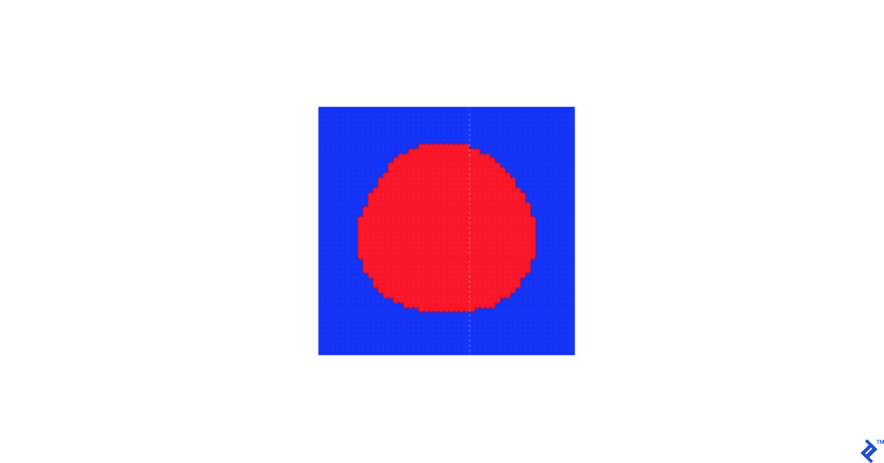
Here, we would like to classify data points on a 2d coordinate system depending on whether they fall within a particular region—a circle of radius 0.5 centered at the origin.

Of course, this can be concretely verified by just checking for a given point (a,b) if a^2 + b^2 < 0.5, but for the purposes of this machine learning experiment, we’d like to instead pass in a training set: A series of random points and whether they fall into our intended region. Here’s one way of creating this:

import numpy as np
NO_OF_RANDOM_POINTS = 100
CIRCLE_RADIUS = 0.5
random_spots = np.random.rand(NO_OF_RANDOM_POINTS, 2) * 2 - 1
is_inside_circle = (np.power(random_spots[:,0],2) + np.power(random_spots[:,1],2) < CIRCLE_RADIUS).astype(int)

We’ll make a neural network with the following characteristics:

1. It consists of an input layer with two nodes, in which we feed our series of two-dimensional vectors contained within “random_spots”. This will be represented by a placeholder awaiting the training data.
2. The output layer will also have two nodes, so we need to feed our series of training labels (“is_inside_circle”) into a placeholder for a scalar, and then convert those values into a one-hot two-dimensional vector.
3. We will have one hidden layer consisting of three nodes, so we will need to use variables for our weights matrices and bias vectors, as these are the values that need to be refined when performing the training.

INPUT_LAYER_SIZE = 2
HIDDEN_LAYER_SIZE = 3
OUTPUT_LAYER_SIZE = 2
 
# Starting values for weights and biases are drawn randomly and uniformly from  [-1, 1]
# For example W1 is a matrix of shape 2x3
W1 = tf.Variable(tf.random_uniform([INPUT_LAYER_SIZE, HIDDEN_LAYER_SIZE], -1, 1))
b1 = tf.Variable(tf.random_uniform([HIDDEN_LAYER_SIZE], -1, 1))
W2 = tf.Variable(tf.random_uniform([HIDDEN_LAYER_SIZE, OUTPUT_LAYER_SIZE], -1, 1))
b2 = tf.Variable(tf.random_uniform([OUTPUT_LAYER_SIZE], -1, 1))
# Specifying that the placeholder X can expect a matrix of 2 columns (but any number of rows)
# representing random spots
X = tf.placeholder(tf.float32, [None, INPUT_LAYER_SIZE])
# Placeholder Y can expect integers representing whether corresponding point is in the circle
# or not (no shape specified)
Y = tf.placeholder(tf.uint8)
# An op to convert to a one hot vector
onehot_output = tf.one_hot(Y, OUTPUT_LAYER_SIZE)

To complete the definition of our graph, we define some ops which will help us train the variables to reach a better classifier. These include the matrix calculations, activation functions, and optimizer.

LEARNING_RATE = 0.01
# Op to perform matrix calculation X*W1 + b1
hidden_layer = tf.add(tf.matmul(X, W1), b1)
# Use sigmoid activation function on the outcome
activated_hidden_layer = tf.sigmoid(hidden_layer)
# Apply next weights and bias (W2, b2) to hidden layer and then apply softmax function
# to get our output layer (each vector adding up to 1)
output_layer = tf.nn.softmax(tf.add(tf.matmul(activated_hidden_layer, W2), b2))
# Calculate cross entropy for our loss function
loss = -tf.reduce_sum(onehot_output * tf.log(output_layer))
# Use gradient descent optimizer at specified learning rate to minimize value given by loss tensor
train_step = tf.train.GradientDescentOptimizer(LEARNING_RATE).minimize(loss)

Having set up our graph, it’s time to set up a session and run the “train_step” (which also runs any prerequisite ops). Some of these ops use placeholders, so values for those need to be provided. This training step represents one epoch in our learning algorithm and, as such, is looped over the number of epochs we wish to run. We can run other parts of the graph, such as the “loss” tensor for informational purposes.

EPOCH_COUNT = 1000
sess = tf.Session()
tf.global_variables_initializer().run()
for i in range(EPOCH_COUNT):
    if i%100 == 0:
    	print('Loss after %d runs: %f' % (i, sess.run(loss, feed_dict={X: random_spots, Y: is_inside_circle})))
	sess.run(train_step, feed_dict={X: random_spots, Y: is_inside_circle})
print('Final loss after %d runs: %f' % (i, sess.run(loss, feed_dict={X: random_spots, Y: is_inside_circle})))

Once we have trained the algorithm, we can feed in a point and get the output of the neural network like so:

sess.run(output_layer, feed_dict={X: [[1, 1]]}) # Hopefully something close to [1, 0]
sess.run(output_layer, feed_dict={X: [[0, 0]]}) # Hopefully something close to [0, 1]

We can classify the point as out of the circle if the first member of the output vector is greater than 0.5, inside otherwise.

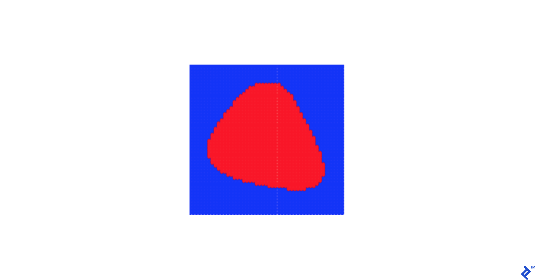
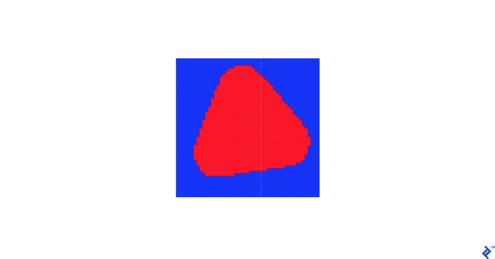
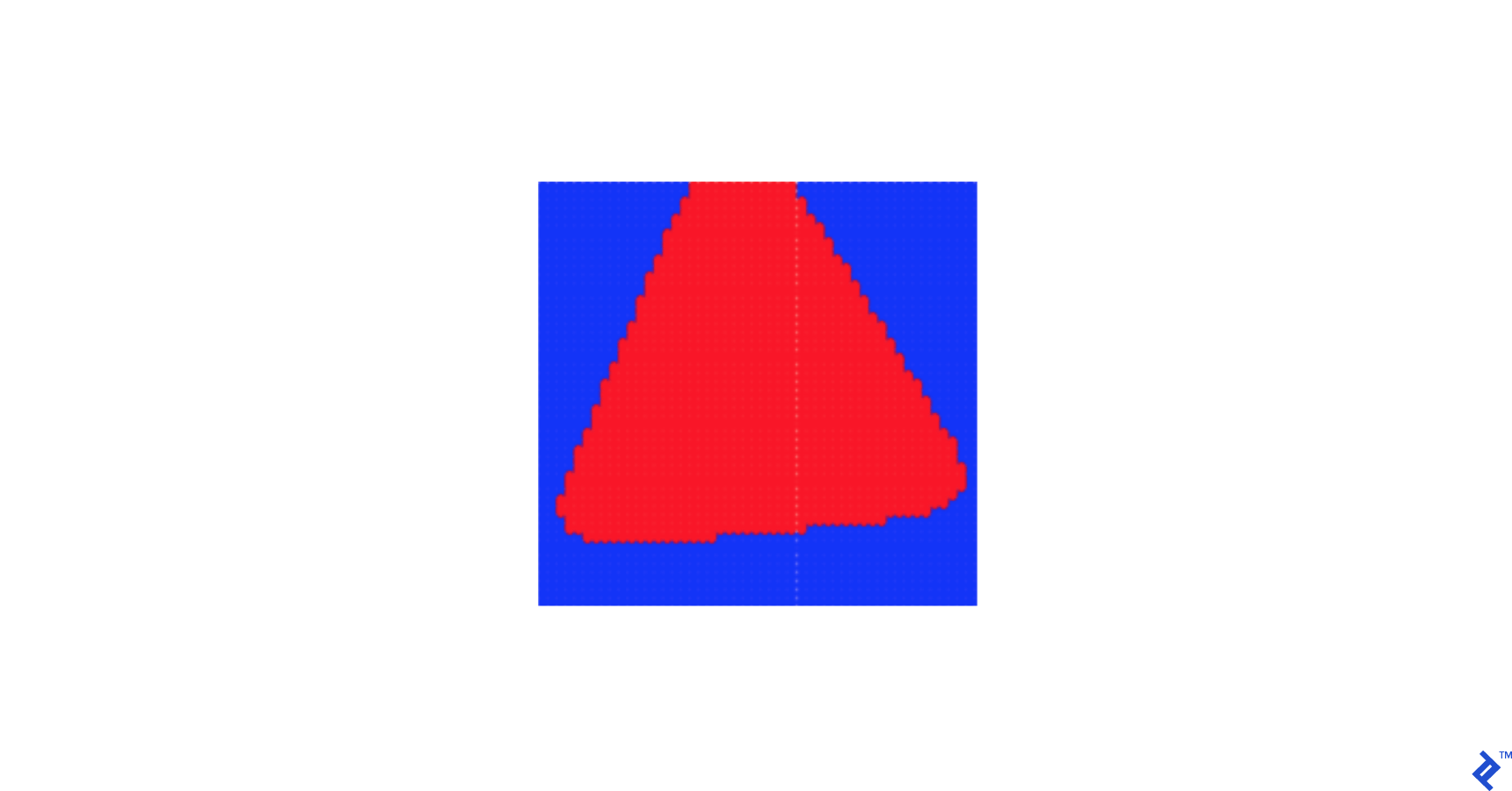
By running the output_layer tensor for many points, we can get an idea of how the learner envisages the region containing the positively classified points. It’s worth playing around with the size of the training set, the learning rate, and other parameters to see how close we can get to the circle we intended.

Wrap Up

This is a good lesson that an increased training set or epoch amount is no guarantee for a good learner—the learning rate should be appropriately adjusted.

Hopefully, these demonstrations have given you a good insight into the core principles of TensorFlow, and provide a solid foundation in which to implement more complex techniques.

We haven’t covered concepts such as the Tensorboard or training our models across GPUs, but these are well-covered in the TensorFlow documentation. A number of recipes can be found in the documentation that can help you get up to speed with tackling exciting deep learning tasks using this powerful framework!