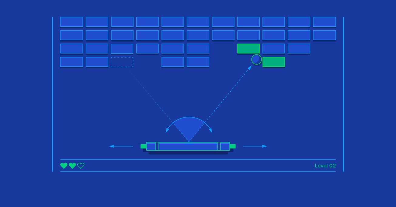
Video Game Physics Tutorial - Part II: Collision Detection for Solid Objects
In Part I of this three-part series on game physics, we explored rigid bodies and their motions. In that discussion, however, objects did not interact with each other. Without some additional work, the simulated rigid bodies can go right through each other.
In Part II, we will cover the collision detection step, which consists of finding pairs of bodies that are colliding among a possibly large number of bodies scattered around a 2D or 3D world.
Nilson (dual BCS/BScTech) been an iOS dev and 2D/3D artist for 8+ years, focusing on physics and vehicle simulations, games, and graphics.
Expertise
This is Part II of our three-part series on video game physics. For the rest of this series, see:
Part I: An Introduction to Rigid Body Dynamics
Part III: Constrained Rigid Body Simulation
In Part I of this series, we explored rigid bodies and their motions. In that discussion, however, objects did not interact with each other. Without some additional work, the simulated rigid bodies can go right through each other, or “interpenetrate”, which is undesirable in the majority of cases.
In order to more realistically simulate the behavior of solid objects, we have to check if they collide with each other every time they move, and if they do, we have to do something about it, such as applying forces that change their velocities, so that they will move in the opposite direction. This is where understanding collision physics is particularly important for game developers.
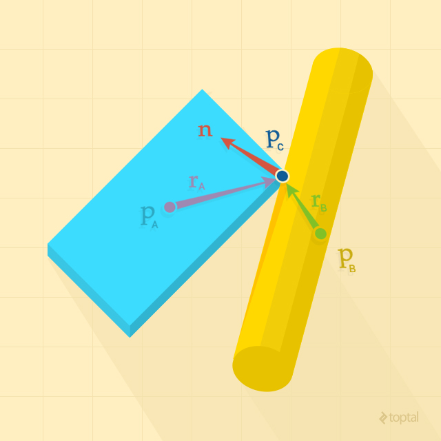
In Part II, we will cover the collision detection step, which consists of finding pairs of bodies that are colliding among a possibly large number of bodies scattered around a 2D or 3D world. In the next, and final, installment, we’ll talk more about “solving” these collisions to eliminate interpenetrations.
For a review of the linear algebra concepts referred to in this article, you can refer to the linear algebra crash course in Part I.
Collision Physics in Video Games
In the context of rigid body simulations, a collision happens when the shapes of two rigid bodies are intersecting, or when the distance between these shapes falls below a small tolerance.
If we have n bodies in our simulation, the computational complexity of detecting collisions with pairwise tests is O(n2), a number that makes computer scientists cringe. The number of pairwise tests increases quadratically with the number of bodies, and determining if two shapes, in arbitrary positions and orientations, are colliding is already not cheap. In order to optimize the collision detection process, we generally split it in two phases: broad phase and narrow phase.
The broad phase is responsible for finding pairs of rigid bodies that are potentially colliding, and excluding pairs that are certainly not colliding, from amongst the whole set of bodies that are in the simulation. This step must be able to scale really well with the number of rigid bodies to make sure we stay well under the O(n2) time complexity. To achieve that, this phase generally uses space partitioning coupled with bounding volumes that establish an upper bound for collision.

The narrow phase operates on the pairs of rigid bodies found by the broad phase that might be colliding. It is a refinement step where we determine if the collisions are actually happening, and for each collision that is found, we compute the contact points that will be used to solve the collisions later.

In the next sections we’ll talk about some algorithms that can be used in the broad phase and narrow phase.
Broad Phase
In the broad phase of collision physics for video games we need to identify which pairs of rigid bodies might be colliding. These bodies might have complex shapes like polygons and polyhedrons, and what we can do to accelerate this is to use a simpler shape to encompass the object. If these bounding volumes do not intersect, then the actual shapes also do not intersect. If they intersect, then the actual shapes might intersect.
Some popular types of bounding volumes are oriented bounding boxes (OBB), circles in 2D, and spheres in 3D. Let’s look at one of the simplest bounding volumes: axis-aligned bounding boxes (AABB).

AABBs get a lot of love from physics programmers because they are simple and offer good tradeoffs. A 2-dimensional AABB may be represented by a struct like this in the C language:
typedef struct {
    float x;
    float y;
} Vector2;

typedef struct {
    Vector2 min;
    Vector2 max;
} AABB;
The min field represents the location of the lower left corner of the box and the max field represents the top right corner.

To test if two AABBs intersect, we only have to find out if their projections intersect on all of the coordinate axes:
BOOL TestAABBOverlap(AABB* a, AABB* b)
{
    float d1x = b->min.x - a->max.x;
    float d1y = b->min.y - a->max.y;
    float d2x = a->min.x - b->max.x;
    float d2y = a->min.y - b->max.y;

    if (d1x > 0.0f || d1y > 0.0f)
        return FALSE;

    if (d2x > 0.0f || d2y > 0.0f)
        return FALSE;

    return TRUE;
}
This code has the same logic of the b2TestOverlap function from the Box2D engine (version 2.3.0). It calculates the difference between the min and max of both AABBs, in both axes, in both orders. If any of these values is greater than zero, the AABBs don’t intersect.
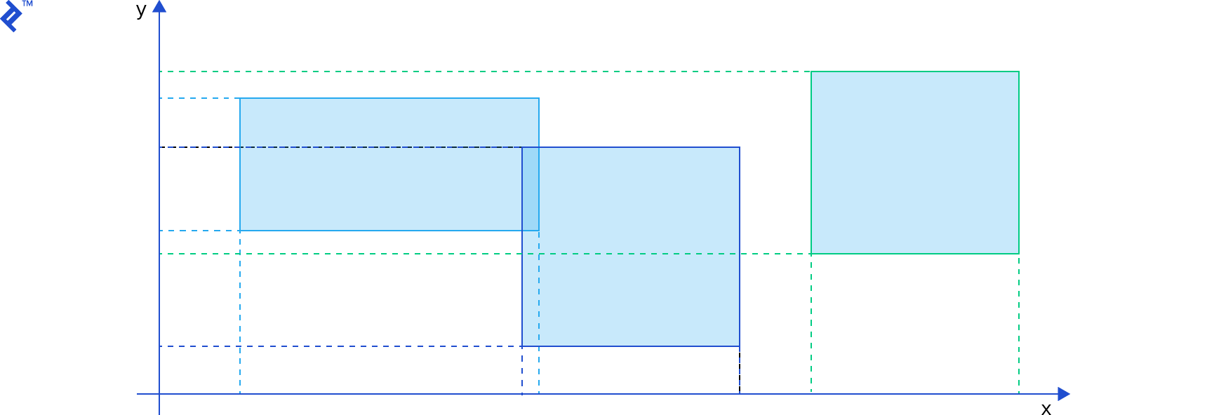
Even though an AABB overlap test is cheap, it won’t help much if we still do pairwise tests for every possible pair since we still have the undesirable O(n2) time complexity. To minimize the number of AABB overlap tests we can use some kind of space partitioning, which which works on the same principles as database indices that speed up queries. (Geographical databases, such as PostGIS, actually use similar data structures and algorithms for their spatial indexes.) In this case, though, the AABBs will be moving around constantly, so generally, we must recreate indices after every step of the simulation.
There are plenty of space partitioning algorithms and data structures that can be used for this, such as uniform grids, quadtrees in 2D, octrees in 3D, and spatial hashing. Let us take a closer look at two popular spatial partitioning algorithms: sort and sweep, and bounding volume hierarchies (BVH).
The Sort and Sweep Algorithm
The sort and sweep method (alternatively known as sweep and prune) is one of the favorite choices among physics programmers for use in rigid body simulation. The Bullet Physics engine, for example, has an implementation of this method in the btAxisSweep3 class.
The projection of one AABB onto a single coordinate axis is essentially an interval [b, e] (that is, beginning and end). In our simulation, we’ll have many rigid bodies, and thus, many AABBs, and that means many intervals. We want to find out which intervals are intersecting.
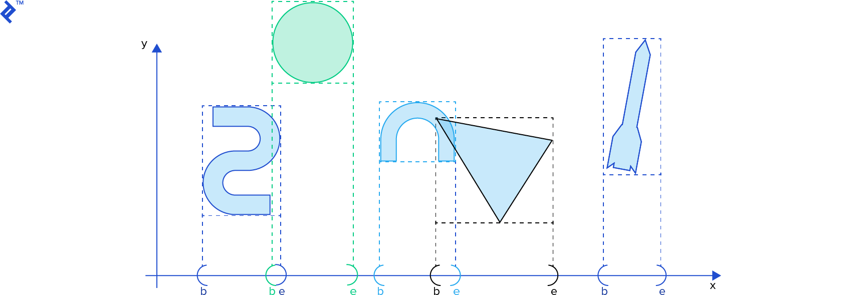
In the sort and sweep algorithm, we insert all b and e values in a single list and sort it ascending by their scalar values. Then we sweep or traverse the list. Whenever a b value is encountered, its corresponding interval is stored in a separate list of active intervals, and whenever an e value is encountered, its corresponding interval is removed from the list of active intervals. At any moment, all the active intervals are intersecting. (Check out David Baraff’s Ph. D Thesis, p. 52 for details. I suggest using this online tool to view the postscript file.) The list of intervals can be reused on each step of the simulation, where we can efficiently re-sort this list using insertion sort, which is good at sorting nearly-sorted lists.
In two and three dimensions, running the sort and sweep, as described above, over a single coordinate axis will reduce the number of direct AABB intersection tests that must be performed, but the payoff may be better over one coordinate axis than another. Therefore, more sophisticated variations of the sort and sweep algorithm are implemented. In his book Real-Time Collision Detection (page 336), Christer Ericson presents an efficient variation where he stores all AABBs in a single array, and for each run of the sort and sweep, one coordinate axis is chosen and the array is sorted by the min value of the AABBs in the chosen axis, using quicksort. Then, the array is traversed and AABB overlap tests are performed. To determine the next axis that should be used for sorting, the variance of the center of the AABBs is computed, and the axis with greater variance is chosen for the next step.
Dynamic Bounding Volume Trees
Another useful spatial partitioning method is the dynamic bounding volume tree, also known as Dbvt. This is a type of bounding volume hierarchy.
The Dbvt is a binary tree in which each node has an AABB that bounds all the AABBs of its children. The AABBs of the rigid bodies themselves are located in the leaf nodes. Typically, a Dbvt is “queried” by giving the AABB for which we would like to detect intersections. This operation is efficient because the children of nodes that do not intersect the queried AABB do not need to be tested for overlap. As such, an AABB collision query starts from the root, and continues recursively through the tree only for AABB nodes that intersect with the queried AABB. The tree can be balanced through tree rotations, as in an AVL tree.
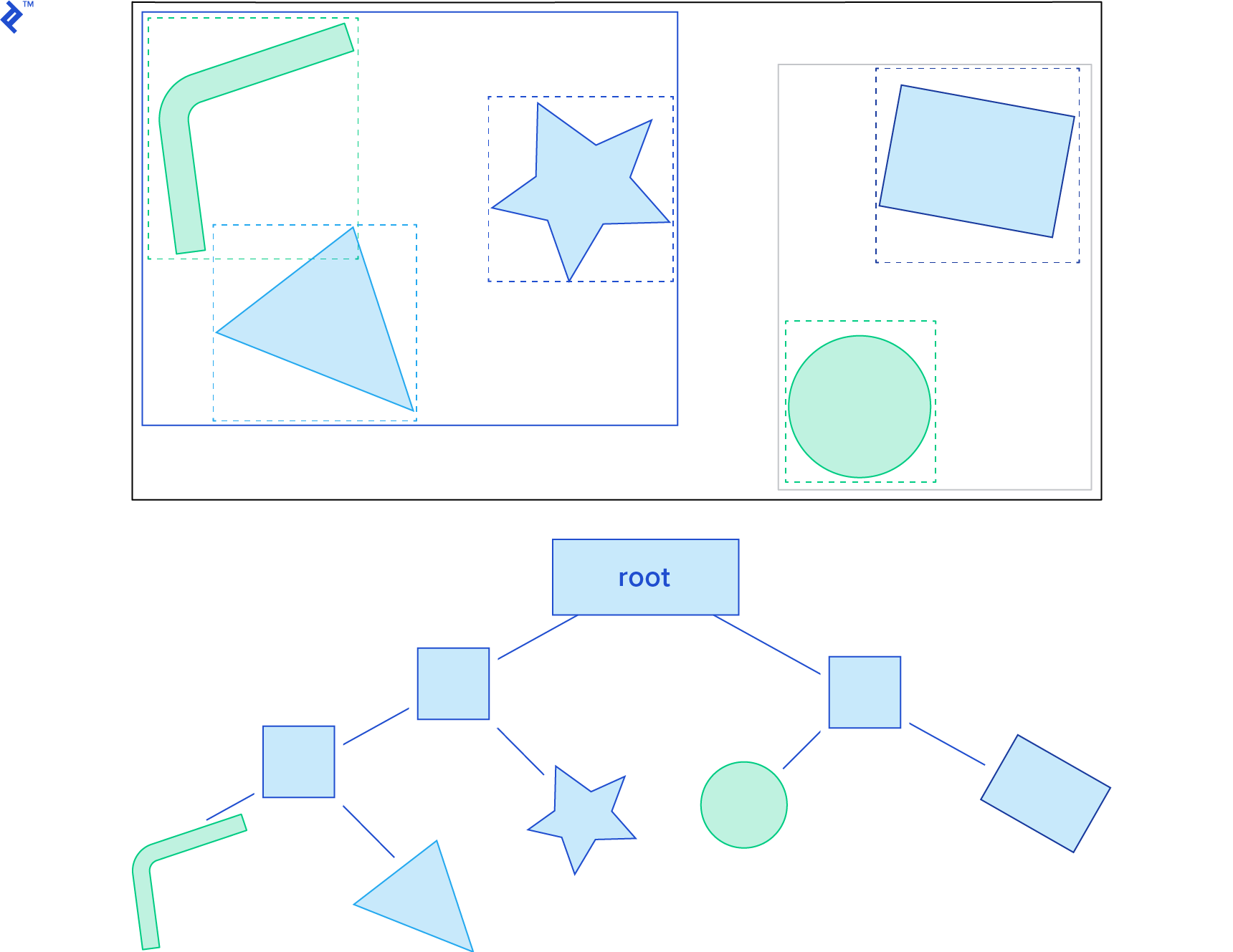
Box2D has a sophisticated implementation of Dbvt in the b2DynamicTree class. The b2BroadPhase class is responsible for performing the broad phase, and it uses an instance of b2DynamicTree to perform AABB queries.
Narrow Phase
After the broad phase of video game collision physics, we have a set of pairs of rigid bodies that are potentially colliding. Thus, for each pair, given the shape, position and orientation of both bodies, we need to find out if they are, in fact, colliding; if they are intersecting or if their distance falls under a small tolerance value. We also need to know what points of contact are between the colliding bodies, since this is needed to resolve the collisions later.
Convex and Concave Shapes
As a video game physics general rule, it is not trivial to determine if two arbitrary shapes are intersecting, or to compute the distance between them. However, one property that is of critical importance in determining just how hard it is, is the convexity of the shape. Shapes can be either convex or concave and concave shapes are harder to work with, so we need some strategies to deal with them.
In a convex shape, a line segment between any two points within the shape always falls completely inside the shape. However for a concave (or “non-convex”) shape, the same is not true for all possible line segments connecting points in the shape. If you can find at least one line segment that falls outside of the shape at all, then the shape is concave.

Computationally, it is desirable that all shapes are convex in a simulation, since we have a lot of powerful distance and intersection test algorithms that work with convex shapes. Not all objects will be convex though, and usually we work around them in two ways: convex hull and convex decomposition.
The convex hull of a shape is the smallest convex shape that fully contains it. For a concave polygon in two dimensions, it would be like hammering a nail on each vertex and wrapping a rubber band around all nails. To calculate the convex hull for a polygon or polyhedron, or more generally, for a set of points, a good algorithm to use is the quickhull algorithm, which has an average time complexity of O(n log n).

Obviously, if we use a convex hull to represent a concave object, it will lose its concave properties. Undesirable behavior, such as “ghost” collisions may become apparent, since the object will still have a concave graphical representation. For example, a car usually has a concave shape, and if we use a convex hull to represent it physically and then put a box on it, the box might appear to be floating in the space above.

In general, convex hulls are often good enough to represent concave objects, either because the unrealistic collisions are not very noticeable, or their concave properties are not essential for whatever is being simulated. In some cases, though, we might want to have the concave object behave like a concave shape physically. For example, if we use a convex hull to represent a bowl physically, we won’t be able to put anything inside of it. Objects will just float on top of it. In this case, we can use a convex decomposition of the concave shape.
Convex decomposition algorithms receive a concave shape and return a set of convex shapes whose union is identical to the original concave shape. Some concave shapes can only be represented by a large number of convex shapes, and these might become prohibitively costly to compute and use. However, an approximation is often good enough, and so, algorithms such as V-HACD produce a small set of convex polyhedrons out of a concave polyhedron.
In many collisons physics cases, though, the convex decomposition can be made by hand, by an artist. This eliminates the need to tax performance with decomposition algorithms. Since performance is one of the most important aspects in real-time simulations, it’s generally a good idea to create very simple physical representations for complex graphic objects. The image below shows one possible convex decomposition of a 2D car using nine convex shapes.

Testing for Intersections - The Separating Axis Theorem
The separating axis theorem (SAT) states that two convex shapes are not intersecting if and only if there exists at least one axis where the orthogonal projections of the shapes on this axis do not intersect.

It’s usually more visually intuitive to find a line in 2D or a plane in 3D that separates the two shapes, though, which is effectively the same principle. A vector orthogonal to the line in 2D, or the normal vector of the plane in 3D, can be used as the “separating axis”.

Game physics engines have a number of different classes of shapes, such as circles (spheres in 3D), edges (a single line segment), and convex polygons (polyhedrons in 3D). For each pair of shape type, they have a specific collision detection algorithm. The simplest of them is probably the circle-circle algorithm:
typedef struct {
    float centerX;
    float centerY;
    float radius;
} Circle;

bool CollideCircles(Circle *cA, Circle *cB) {
    float x = cA->centerX - cB->centerX;
    float y = cA->centerY - cB->centerY;
    float centerDistanceSq = x * x + y * y; // squared distance
    float radius = cA->radius + cB->radius;
    float radiusSq = radius * radius;
    return centerDistanceSq <= radiusSq;
}
Even though the SAT applies to circles, it’s much simpler to just check if the distance between their centers is smaller than the sum of their radii. For that reason, the SAT is used in the collision detection algorithm for specific pairs of shape classes, such as convex polygon against convex polygon (or polyhedrons in 3D).
For any pair of shapes, there are an infinite number of axes we can test for separation. Thus, determining which axis to test first is crucial for an efficient SAT implementation. Fortunately, when testing if a pair of convex polygons collide, we can use the edge normals as potential separating axes. The normal vector n of an edge is perpendicular to the edge vector, and points outside the polygon. For each edge of each polygon, we just need to find out if all the vertices of the other polygon are in front of the edge.
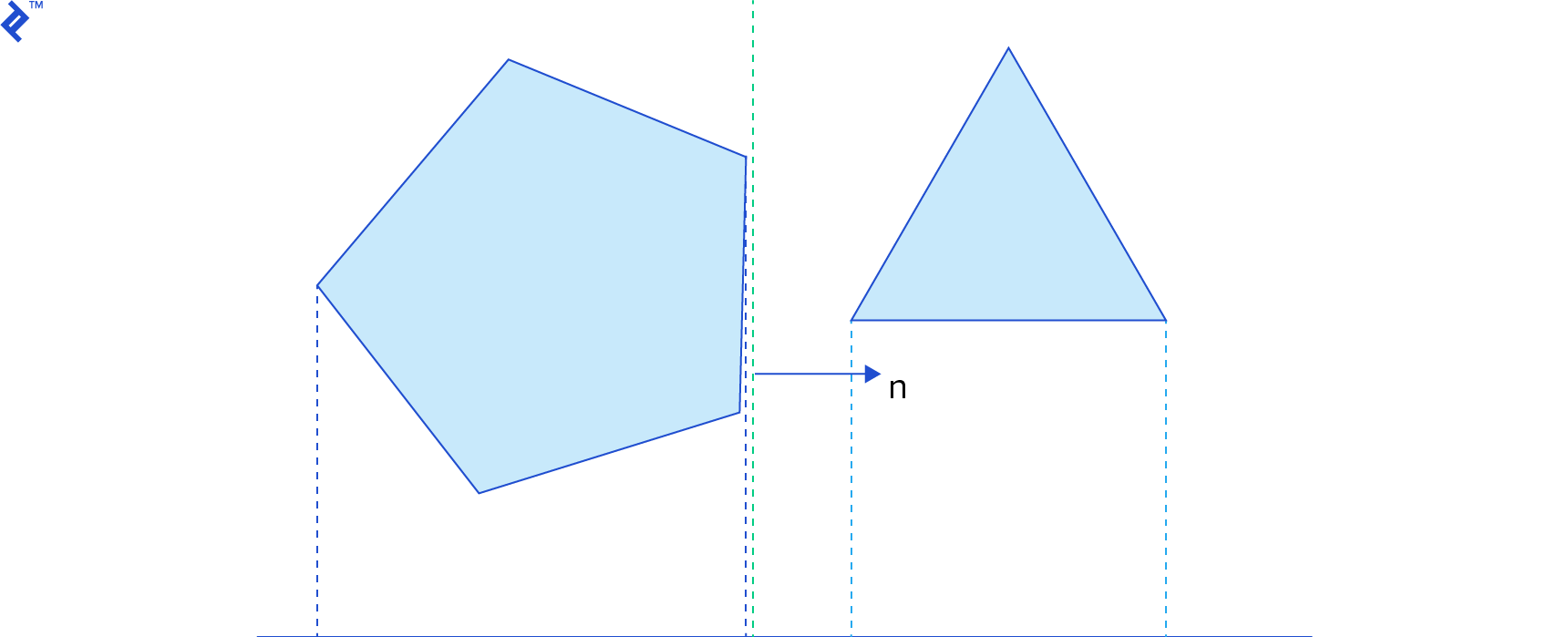
If any test passes – that is, if, for any edge, all vertices of the other polygon are in front of it – then the polygons do not intersect. Linear algebra provides an easy formula for this test: given an edge on the first shape with vertices a and b and a vertex v on the other shape, if (v - a) · n is greater than zero, then the vertex is in front of the edge.
For polyhedrons, we can use the face normals and also the cross product of all edge combinations from each shape. That sounds like a lot of things to test; however, to speed things up, we can cache the last separating axis we used and try using it again in the next steps of the simulation. If the cached separating axis does not separate the shapes anymore, we can search for a new axis starting from faces or edges that are adjacent to the previous face or edge. That works because the bodies often don’t move or rotate much between steps.
Box2D uses SAT to test if two convex polygons are intersecting in its polygon-polygon collision detection algorithm in b2CollidePolygon.cpp.
Computing Distance - The Gilbert-Johnson-Keerthi Algorithm
In many collisions physics cases, we want to consider objects to be colliding not only if they are actually intersecting, but also if they are very close to each other, which requires us to know the distance between them. The Gilbert-Johnson-Keerthi (GJK) algorithm computes the distance between two convex shapes and also their closest points. It is an elegant algorithm that works with an implicit representation of convex shapes through support functions, Minkowski sums, and simplexes, as explained below.
Support Functions
A support function sA(d) returns a point on the boundary of the shape A that has the highest projection on the vector d. Mathematically, it has the highest dot product with d. This is called a support point, and this operation is also known as support mapping. Geometrically, this point is the farthest point on the shape in the direction of d.
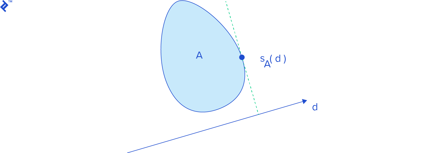
Finding a support point on a polygon is relatively easy. For a support point for vector d, you just have to loop through its vertices and find the one which has the highest dot product with d, like this:
Vector2 GetSupport(Vector2 *vertices, int count, Vector2 d) {
    float highest = -FLT_MAX;
    Vector2 support = (Vector2){0, 0};

    for (int i = 0; i < count; ++i) {
        Vector2 v = vertices[i];
        float dot = v.x * d.x + v.y * d.y;

        if (dot > highest) {
            highest = dot;
            support = v;
        }
    }

    return support;
}
However, the real power of a support function is that makes it easy to work with shapes such as cones, cylinders, and ellipses, among others. It is rather difficult to compute the distance between such shapes directly, and without an algorithm like GJK you would usually have to discretize them into a polygon or polyhedron to make things simpler. However, that might lead to further problems because the surface of a polyhedron is not as smooth as the surface of, say, a sphere, unless the polyhedron is very detailed, which can lead to poor performance during collision detection. Other undesirable side effects might show up as well; for example, a “polyhedral” sphere might not roll smoothly.
To get a support point for a sphere centered on the origin, we just have to normalize d (that is, compute d / ||d||, which is a vector with length 1 (unit length) that still points in the same direction of d) and then we multiply it by the sphere radius.
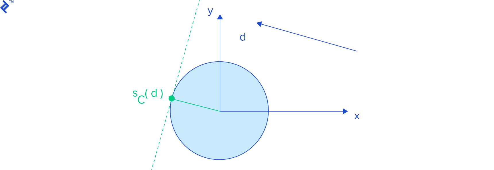
Check Gino van den Bergen’s paper to find more examples of support functions for cylinders, and cones, among other shapes.
Our objects will, of course, be displaced and rotated from the origin in the simulation space, so we need to be able to compute support points for a transformed shape. We use an affine transformation T(x) = Rx + c to displace and rotate our objects, where c is the displacement vector and R is the rotation matrix. This transformation first rotates the object about the origin, and then translates it. The support function for a transformed shape A is:

Minkowski Sums
The Minkowski sum of two shapes A and B is defined as:

That means we compute the sum for all points contained in A and B. The result is like inflating A with B.
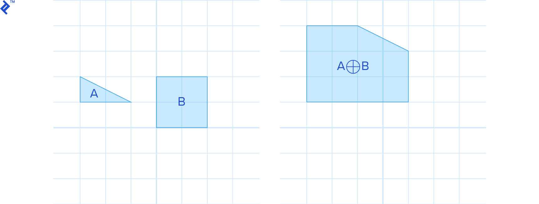
Similarly, we define the Minkowski difference as:

which we can also write as the Minkowski sum of A with -B:

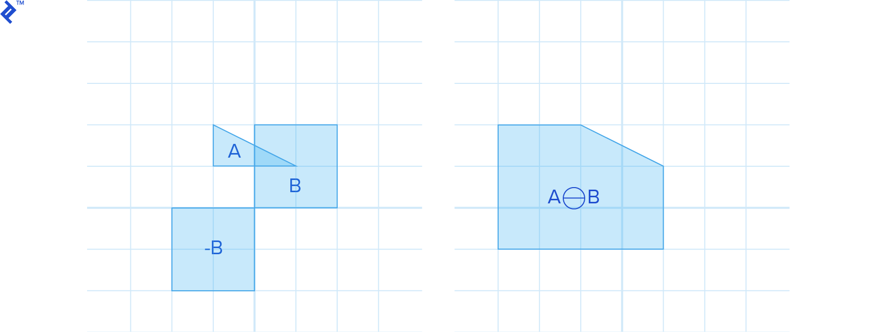
For convex A and B, A⊕B is also convex.
One useful property of the Minkowski difference is that if it contains the origin of the space, the shapes intersect, as can be seen in the previous image. Why is that? Because if two shapes intersect, they have at least one point in common, which lie in the same location in space, and their difference is the zero vector, which is actually the origin.
Another nice feature of the Minkowski difference is that if it doesn’t contain the origin, the minimum distance between the origin and the Minkowski difference is the distance between the shapes.
The distance between two shapes is defined as:

In other words, the distance between A and B is the length of the shortest vector that goes from A to B. This vector is contained in A⊖B and it is the one with the smallest length, which consequently is the one closest to the origin.
It is generally not simple to explicitly build the Minkowski sum of two shapes. Fortunately, we can use support mapping here as well, since:

Simplexes
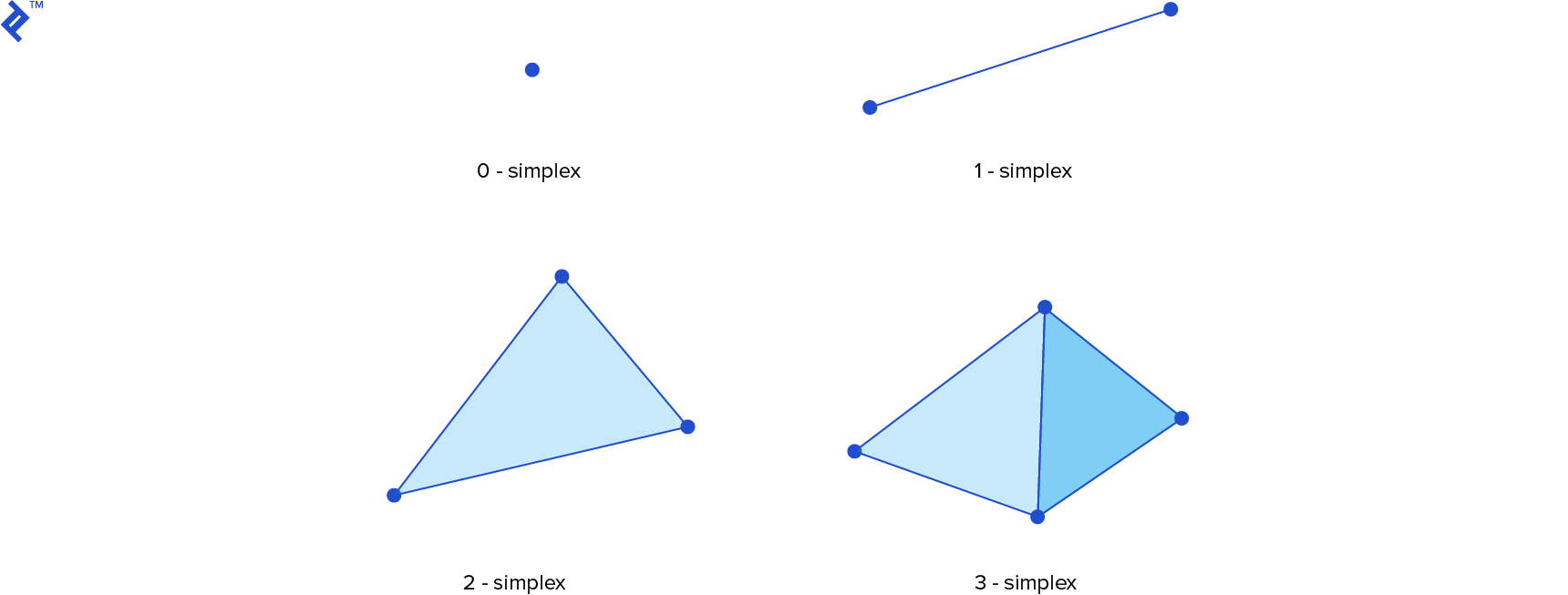
The GJK algorithm iteratively searches for the point on the Minkowski difference closest to the origin. It does so by building a series of simplexes that are closer to the origin in each iteration. A simplex – or more specifically, a k-simplex for an integer k – is the convex hull of k + 1 affinely independent points in a k-dimensional space. That is, if for two points, they must not coincide, for three points they additionally must not lie on the same line, and if we have four points they also must not lie on the same plane. Hence, the 0-simplex is a point, the 1-simplex is a line segment, the 2-simplex is a triangle and the 3-simplex is a tetrahedron. If we remove a point from a simplex we decrement its dimensionality by one, and if we add a point to a simplex we increment its dimensionality by one.
GJK in Action
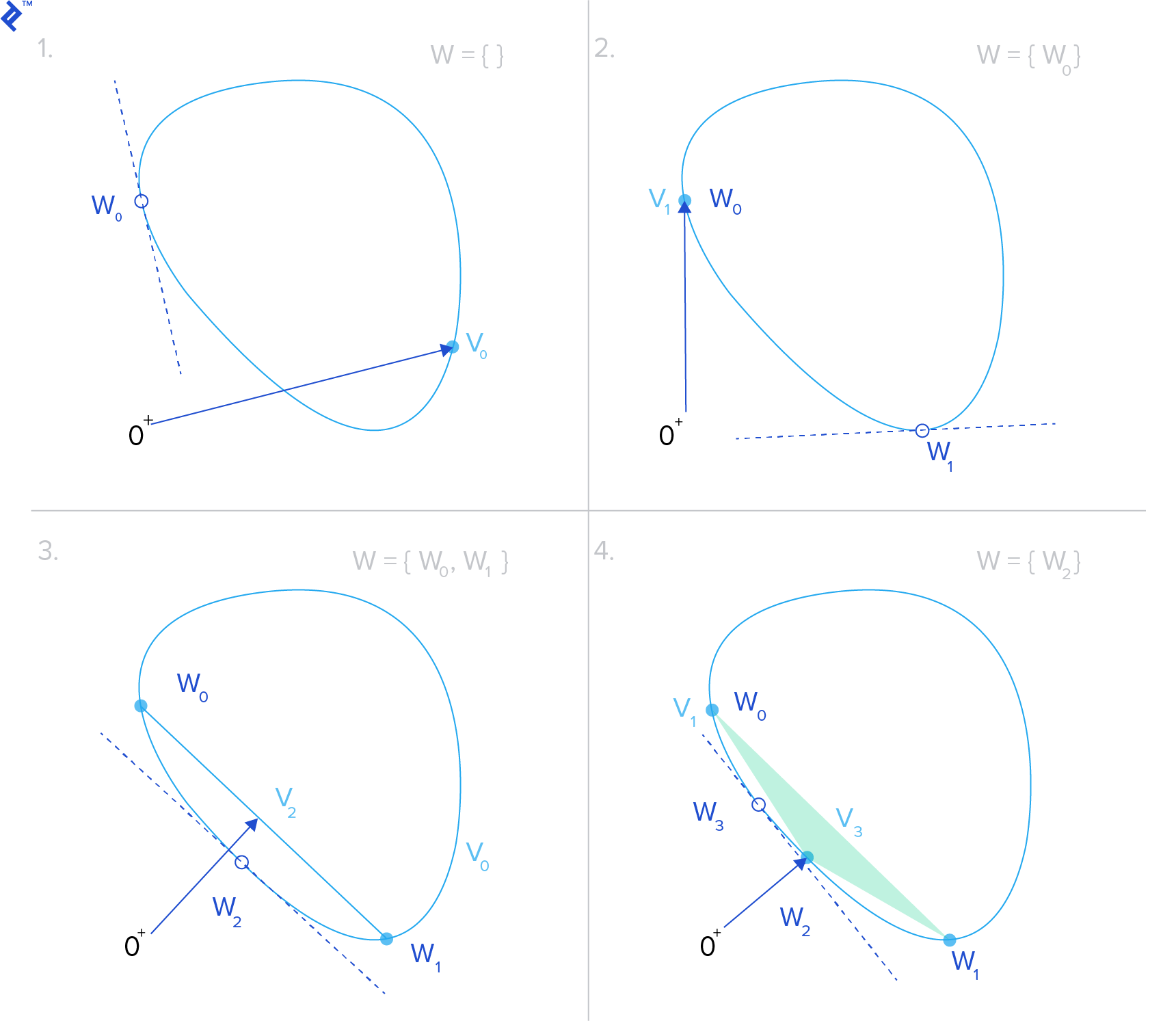
Let’s put this all together to see how GJK works. To determine the distance between two shapes A and B, we start by taking their Minkowski difference A⊖B. We are searching for the closest point to the origin on the resulting shape, since the distance to this point is the distance between the original two shapes. We choose some point v in A⊖B, which will be our distance approximation. We also define an empty point set W, which will contain the points in the current test simplex.
Then we enter a loop. We start by getting the support point w = sA⊖B(-v), the point on A⊖B whose projection onto v is closest to the origin.
If ||w|| is not much different than ||v|| and the angle between them didn’t change much (according to some predefined tolerances), it means the algorithm has converged and we can return ||v|| as the distance.
Otherwise, we add w to W. If the convex hull of W (that is, the simplex) contains the origin, the shapes intersect, and this also means we are done. Otherwise, we find the point in the simplex that is closest to the origin and then we reset v to be this new closest approximation. Finally, we remove whatever points in W that do not contribute to the closest point computation. (For example, if we have a triangle, and the closest point to the origin lies in one of its edges, we can remove the point from W that is not a vertex of this edge.) Then we repeat these same steps until the algorithm converges.
The next image shows an example of four iterations of the GJK algorithm. The blue object represents the Minkowski difference A⊖B and the green vector is v. You can see here how v hones in on the closest point to the origin.
For a detailed and in-depth explanation of the GJK algorithm, check out the paper A Fast and Robust GJK Implementation for Collision Detection of Convex Objects, by Gino van den Bergen. The blog for the dyn4j physics engine also has a great post on GJK.
Box2D has an implementation of the GJK algorithm in b2Distance.cpp, in the b2Distance function. It only uses GJK during time of impact computation in its algorithm for continuous collision detection (a topic we will discuss further down).
The Chimpunk physics engine uses GJK for all collision detection, and its implementation is in cpCollision.c, in the GJK function. If the GJK algorithm reports intersection, it still needs to know what the contact points are, along with the penetration depth. To do that, it uses the Expanding Polytope Algorithm, which we shall explore next.
Determining Penetration Depth - The Expanding Polytope Algorithm
As stated above, if the shapes A and B are intersecting, GJK will generate a simplex W that contains the origin, inside the Minkowski difference A⊖B. At this stage, we only know that the shapes intersect, but in the design of many collision detection systems, it is desirable to be able to compute how much intersection we have, and what points we can use as the points of contact, so that we handle the collision in a realistic way. The Expanding Polytope Algorithm (EPA) allows us to obtain that information, starting where GJK left off: with a simplex that contains the origin.
The penetration depth is the length of the minimum translation vector (MTV), which is the smallest vector along which we can translate an intersecting shape to separate it from the other shape.
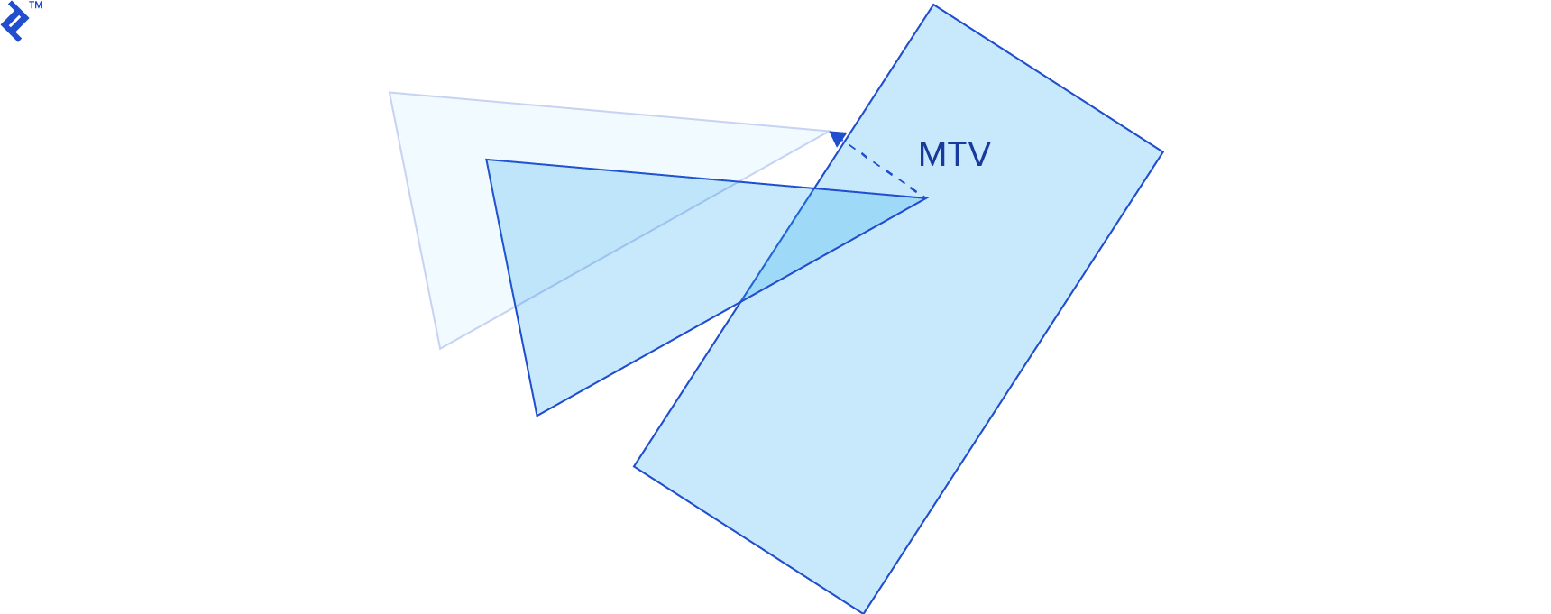
When two shapes are intersecting, their Minkowski difference contains the origin, and the point on the boundary of the Minkowski difference that is closest to the origin is the MTV. The EPA algorithm finds that point by expanding the simplex that GJK gave us into a polygon; successively subdividing it’s edges with new vertices.
First, we find the edge of the simplex closest to the origin, and compute the support point in the Minkowski difference in a direction that is normal to the edge (i.e. perpendicular to it and pointing outside the polygon). Then we split this edge by adding this support point to it. We repeat these steps until the length and direction of the vector doesn’t change much. Once the algorithm converges, we have the MTV and the penetration depth.

Using GJK in combination with EPA, we get a detailed description of the collision, no matter if the objects are already intersecting, or just close enough to be considered a collision.
The EPA algorithm is described in the paper Proximity Queries and Penetration Depth Computation on 3D Game Objects, also written by Gino van den Bergen. The dyn4j blog also has a post about EPA.
Continuous Collision Detection
The video game physics techniques presented so far perform collision detection for a static snapshot of the simulation. This is called discrete collision detection, and it ignores what happens between the previous and current steps. For this reason, some collisions might not be detected, especially for fast moving objects. This issue is known as tunneling.

Continuous collision detection techniques attempt to find when two bodies collided between the previous and the current step of the simulation. They compute the time of impact, so we can then go back in time and process the collision at that point.
The time of impact (or time of contact) tc is the instant of time when the distance between two bodies is zero. If we can write a function for the distance between two bodies along time, what we want to find is the smallest root of this function. Thus, the time of impact computation is a root-finding problem.
For the time of impact computation, we consider the state (position and orientation) of the body in the previous step at time ti-1, and in the current step at time ti. To make things simpler, we assume linear motion between the steps.
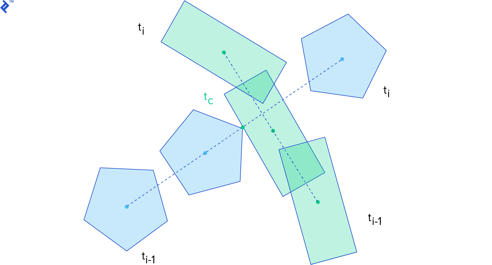
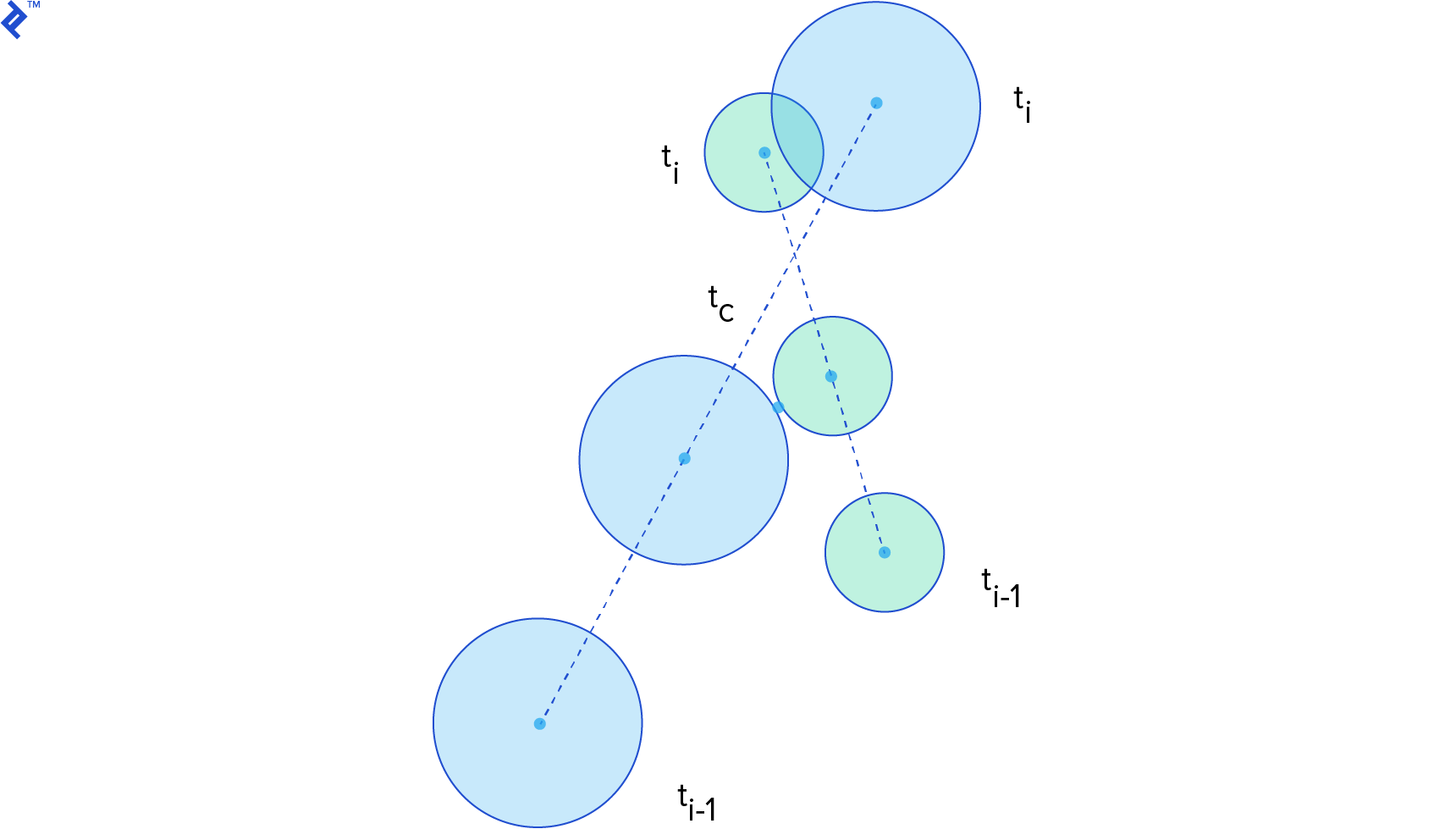
Let’s simplify the problem by assuming the shapes are circles. For two circles C1 and C2, with radius r1 and r2, where their center of mass x1 and x2 coincide with their centroid (i.e., they naturally rotate about their center of mass), we can write the distance function as:

Considering linear motion between steps, we can write the following function for the position of C1 from ti-1 to ti

It is a linear interpolation from x1(ti-1) to x1(ti). The same can be done for x2. For this interval we can write another distance function:

Set this expression equal to zero and you get a quadratic equation on t. The roots can be found directly using the quadratic formula. If the circles don’t intersect, the quadratic formula will not have a solution. If they do, it might result in one or two roots. If it has only one root, that value is the time of impact. If it has two roots, the smallest one is the time of impact and the other is the time when the circles separate. Note that the time of impact here is a number from 0 to 1. It is not a time in seconds; it is just a number we can use to interpolate the state of the bodies to the precise location where the collision happened.
Continuous Collision Detection for Non-Circles
Writing a distance function for other kinds of shapes is difficult, primarily because their distance depends on their orientations. For this reason, we generally use iterative algorithms that move the objects closer and closer on each iteration until they are close enough to be considered colliding.
The conservative advancement algorithm moves the bodies forward (and rotates them) iteratively. In each iteration it computes an upper bound for displacement. The original algorithm is presented in Brian Mirtich’s PhD Thesis (section 2.3.2), which considers the ballistic motion of bodies. This paper by Erwin Coumans (the author of the Bullet Physics Engine) presents a simpler version that uses constant linear and angular velocities.
The algorithm computes the closest points between shapes A and B, draws a vector from one point to the other, and projects the velocity on this vector to compute an upper bound for motion. It guarantees that no points on the body will move beyond this projection. Then it advances the bodies forward by this amount and repeats until the distance falls under a small tolerance value.
It may take too many iterations to converge in some cases, for example, when the angular velocity of one of the bodies is too high.
Resolving Collisions
Once a collision has been detected, it is necessary to change the motions of the colliding objects in a realistic way, such as causing them to bounce off each other. In the next and final installment in this theories, we’ll discuss some popular methods for resolving collisions in video games.
References
If you are interested in obtaining a deeper understanding about collision physics such as collision detection algorithms and techniques, the book Real-Time Collision Detection, by Christer Ericson, is a must-have.
Since collision detection relies heavily on geometry, Toptal’s article Computational Geometry in Python: From Theory to Application is an excellent introduction to the topic.
Further Reading on the Toptal Blog:
- Video Game Physics Tutorial - Part III: Constrained Rigid Body Simulation
- Video Game Physics Tutorial - Part I: An Introduction to Rigid Body Dynamics
- Buggy PHP Code: The 10 Most Common Mistakes PHP Developers Make
- An Introductory Robot Programming Tutorial
- Forex Algorithmic Trading: A Practical Tale for Engineers
Bella Vista, Panama City, Panama, Panama
Member since February 19, 2013
About the author
Nilson (dual BCS/BScTech) been an iOS dev and 2D/3D artist for 8+ years, focusing on physics and vehicle simulations, games, and graphics.
