
Video Game Physics Tutorial - Part I: An Introduction to Rigid Body Dynamics
Simulating physics in video games is very common, since most games are inspired by things we have in the real world. Rigid body dynamics – the movement and interaction of solid, inflexible objects – is by far the most popular kind of effect simulated in games.
In this series, rigid body simulation will be explored, starting with simple rigid body motion in this article, and then covering interactions among bodies through collisions and constraints in the following installments.

Nilson (dual BCS/BScTech) been an iOS dev and 2D/3D artist for 8+ years, focusing on physics and vehicle simulations, games, and graphics.
Expertise
-This is Part I of our three-part series on video game physics. For the rest of this series, see:
Part II: Collision Detection for Solid Objects
Part III: Constrained Rigid Body Simulation
Physics simulation is a field within computer science that aims to reproduce physical phenomena using a computer. In general, these simulations apply numerical methods to existing theories to obtain results that are as close as possible to what we observe in the real world. This allows us, as advanced game developers, to predict and carefully analyze how something would behave before actually building it, which is almost always simpler and cheaper to do.

The range of applications of physics simulations is enormous. The earliest computers were already being used to perform physics simulations – for example, to predict the ballistic motion of projectiles in the military. It is also an essential tool in civil and automotive engineering, illuminating how certain structures would behave in events like an earthquake or a car crash. And it doesn’t stop there. We can simulate things like astrophysics, relativity, and lots of other insane stuff we are able to observe in among the wonders of nature.
Simulating physics in video games is very common, since most games are inspired by things we have in the real world. Many games rely entirely on the physics simulation to be fun. A physics simulation game thus requires a stable simulation that will not break or slow down, and this is usually not trivial to achieve.
In any game, only certain physical effects are of interest. Rigid body dynamics – the movement and interaction of solid, inflexible objects – is by far the most popular kind of effect simulated in games. That’s because most of the objects we interact with in real life are fairly rigid, and simulating rigid bodies is relatively simple (although as we will see, that doesn’t mean it’s a cakewalk). A few other games require the simulation of more complicated entities though, such as deformable bodies, fluids, magnetic objects, etc.
In this tutorial series on physics in games, we’ll explore rigid body physics simulation, starting with simple rigid body motion in this article, and then covering interactions among bodies through collisions and constraints in the following installments. The most common equations used in modern game physics engines such as Box2D, Bullet Physics, Chipmunk Physics, Jolt Physics, Rapier, and PhysX will be presented and explained.
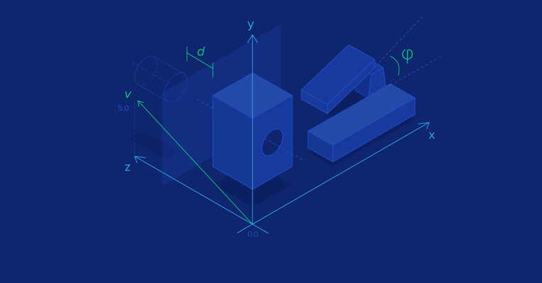
Rigid Body Dynamics
In video game physics, we want to animate objects on screen and give them realistic physical behavior. This is achieved with physics-based procedural animation, which is animation produced by numerical computations applied to the theoretical laws of physics.
Animations are produced by displaying a sequence of images in succession, with objects moving slightly from one image to the next. When the images are displayed in quick succession, the effect is an apparent smooth and continuous movement of the objects. Thus, to animate the objects in a physics simulation, we need to update the physical state of the objects (e.g. position and orientation), according to the laws of physics multiple times per second, and redraw the screen after each update.
The physics engine is the software component that performs the physics simulation. It receives a specification of the bodies that are going to be simulated, plus some configuration parameters, and then the simulation can be stepped. Each step moves the simulation forward by a few fractions of a second, and the results can be displayed on screen afterwards. Note that physics engines only perform the numerical simulation. What is done with the results may depend on the requirements of the game. It is not always the case that the results of every step wants to be drawn to the screen.
The motion of rigid bodies can be modeled using newtonian mechanics, which is founded upon Isaac Newton’s famous Three Laws of Motion:
-
Inertia: If no force is applied on an object, its velocity (speed and direction of motion) shall not change.
-
Force, Mass, and Acceleration: The force acting on an object is equal to the mass of the object multiplied by its acceleration (rate of change of velocity). This is given by the formula F = ma.
-
Action and Reaction: “For every action there is an equal and opposite reaction.” In other words, whenever one body exerts a force on another, the second body exerts a force of the same magnitude and opposite direction on the first.
Based on these three laws, we can make a physics engine that is able to reproduce the dynamic behavior we’re so familiar with, and thus create an immersive experience for the player.
The following diagram shows a high level overview of the general procedure of a physics engine:

Vectors
In order to understand how physics simulations work, it is crucial to have a basic understanding of vectors and their operations. If you are already familiar with vector math, read on. But if you are not, or you want to brush up, take a minute to review the appendix at the end of this article.
Particle Simulation
A good stepping stone to understanding rigid body simulation is to start with particles. Simulating particles is simpler than simulating rigid bodies, and we can simulate the latter using the same principles, but adding volume and shape to the particles. Also, you can easily find good particle physics engine tutorials online, covering various scenarios and levels of realism/complexity.
A particle is just a point in space that has a position vector, a velocity vector and a mass. According to Newton’s First Law, its velocity will only change when a force is applied on it. When its velocity vector has a non-zero length, its position will change over time.
To simulate a particle system, we need to first create an array of particles with an initial state. Each particle must have a fixed mass, an initial position in space and an initial velocity. Then we have to start the main loop of the simulation where, for each particle, we have to compute the force that is currently acting on it, update its velocity from the acceleration produced by the force, and then update its position based on the velocity we just computed.
The force may come from different sources depending on the kind of simulation. It can be gravity, wind, or magnetism, among others – or it can be a combination of these. It can be a global force, such as constant gravity, or it can be a force between particles, such as attraction or repulsion.
To make the simulation run at a realistic pace, the time step we “simulate” should be the same as the real amount of time that passed since the last simulation step. However, this time step can be scaled up to make the simulation run faster, or scaled down to make it run in slow motion.
Suppose we have one particle with mass m, position p(ti) and velocity v(ti) at an instant of time ti. A force f(ti) is applied on that particle at that time. The position and velocity of this particle at a future time ti + 1, p(ti + 1) and v(ti + 1) respectively, can be computed with:

In technical terms, what we’re doing here is numerically integrating an ordinary differential equation of motion of a particle using the semi-implicit Euler method, which is the method most game physics engines use due to its simplicity and acceptable accuracy for small values of the time span, dt. The Differential Equation Basics lecture notes from the amazing Physically Based Modeling: Principles and Practice course, by Drs. Andy Witkin and David Baraff, is a nice article to get a deeper look into the numerical methodology of this method.
The following is an example of a particle simulation in the C language.
#define NUM_PARTICLES 1

// Two dimensional vector.
typedef struct {
    float x;
    float y;
} Vector2;

// Two dimensional particle.
typedef struct {
    Vector2 position;
    Vector2 velocity;
    float mass;
} Particle;

// Global array of particles.
Particle particles[NUM_PARTICLES];

// Prints all particles' position to the output. We could instead
// draw them on screen in a more interesting application.
void PrintParticles() {
    for (int i = 0; i < NUM_PARTICLES; ++i) {
        Particle *particle = &particles[i];
        printf("particle[%i] (%.2f, %.2f)\n", i,
            particle->position.x, particle->position.y);
    }
}

// Initializes all particles with random positions, zero velocities
// and 1kg mass.
void InitializeParticles() {
    for (int i = 0; i < NUM_PARTICLES; ++i) {
        particles[i].position = (Vector2){rand() % 50, rand() % 50};
        particles[i].velocity = (Vector2){0, 0};
        particles[i].mass = 1;
    }
}

// Just applies Earth's gravity force (mass times gravity
// acceleration 9.81 m/s^2) to each particle.
Vector2 ComputeForce(Particle *particle) {
    return (Vector2){0, particle->mass * -9.81};
}

void RunSimulation() {
    float totalSimulationTime = 10; // The simulation will run for
    // 10 seconds.
    float currentTime = 0; // This accumulates the time that has
    // passed.
    float dt = 1; // Each step will take one second.

    srand((unsigned)time(NULL));
    InitializeParticles();
    PrintParticles();

    while (currentTime < totalSimulationTime) {
        // In a real game loop, dt is measured from a
        // high-resolution timer each frame:
        // currentTime = GetTime();
        // dt = currentTime - previousTime;
        // previousTime = currentTime;

        // Production engines usually go a step further and use a
        // fixed-timestep accumulator for stability. For this tutorial we just
        // hold dt constant.

        for (int i = 0; i < NUM_PARTICLES; ++i) {
            Particle *particle = &particles[i];

            Vector2 force = ComputeForce(particle);
            Vector2 acceleration = (Vector2){force.x /
                particle->mass, force.y / particle->mass};

            particle->velocity.x += acceleration.x * dt;
            particle->velocity.y += acceleration.y * dt;

            particle->position.x += particle->velocity.x * dt;
            particle->position.y += particle->velocity.y * dt;
        }

        PrintParticles();
        currentTime += dt;
    }
}
If you call the RunSimulation function (for a single particle) it will print something like:
particle[0] (-8.00, 57.00)
particle[0] (-8.00, 47.19)
particle[0] (-8.00, 27.57)
particle[0] (-8.00, -1.86)
particle[0] (-8.00, -41.10)
particle[0] (-8.00, -90.15)
particle[0] (-8.00, -149.01)
particle[0] (-8.00, -217.68)
particle[0] (-8.00, -296.16)
particle[0] (-8.00, -384.45)
particle[0] (-8.00, -482.55)
As you can see, the particle started at the (-8, 57) position and then its y coordinate started to drop faster and faster, because it was accelerating downwards under the force of gravity.
The following animation gives a visual representation of a sequence of three steps of a single particle being simulated:
Initially, at t = 0, the particle is at p0. After a step it moves in the direction its velocity vector v0 was pointing. In the next step a force f1 is applied to it, and the velocity vector starts to change as if it was being pulled in the direction of the force vector. In the next two steps, the force vector changes direction but continues pulling the particle upwards.
Rigid Body Physics Simulation
A rigid body is a solid that cannot deform. Such solids do not exist in the real world – even the hardest materials deform at least a very small amount when some force is applied to them – but the rigid body is a useful model of physics for game developers that simplifies the study of the dynamics of solids where we can neglect deformations.
A rigid body is like an extension of a particle because it also has mass, position and velocity. Additionally, it has volume and shape, and so it can rotate. That adds more complexity than it sounds, especially in three dimensions.
A rigid body naturally rotates around its center of mass, and the position of a rigid body is considered to be the position of its center of mass. We define the initial state of the rigid body with its center of mass at the origin and a rotation angle of zero. Its position and rotation at any instant of time t is going to be an offset of the initial state.

The center of mass is the mid-point of the mass distribution of a body. If you imagine that a rigid body with mass M is made up of N tiny particles, each with mass mi and location ri inside the body, the center of mass can be computed as:

This formula shows that the center of mass is the average of the particle positions weighted by their mass. If the density of the body is uniform throughout, the center of mass is the same as the geometric center of the body shape, also known as the centroid. Game physics engines usually only support uniform density, so the geometric center can be used as the center of mass.
Rigid bodies are not made up of a finite number of discrete particles though, they’re continuous. For that reason, we should calculate it using an integral instead of a finite sum, like this:

where r is the position vector of each point, and 𝜌 (rho) is a function that gives the density at each point within the body. Essentially, this integral does the same thing as the finite sum, however it does so in a continuous volume V.
Since a rigid body can rotate, we have to introduce its angular properties, which are analogous to a particle’s linear properties. In two dimensions, a rigid body can only rotate about the axis that points out of the screen, hence we only need one scalar to represent its orientation. We usually use radians (which go from 0 to 2π for a full circle) as a unit here instead of angles (that go from 0 to 360 for a full circle), as this simplifies calculations.
In order to rotate, a rigid body needs some angular velocity, which is a scalar with unit radians per second and which is commonly represented by the greek letter ω (omega). However, to gain angular velocity the body needs to receive some rotational force, which we call torque, represented by the greek letter τ (tau). Thus, Newton’s Second Law applied to rotation is:

where α (alpha) is the angular acceleration and I is the moment of inertia.
For rotations, the moment of inertia is analogous to mass for linear motion. It defines how hard it is to change the angular velocity of a rigid body. In two dimensions it is a scalar and is defined as:

where V means that this integral should be performed for all points throughout body volume, r is the position vector of each point relative to the axis of rotation, r2 is actually the dot product of r with itself, and 𝜌 is a function that gives the density at each point within the body.
For example, the moment of inertia of a 2-dimensional box with mass m, width w and height h about its centroid is:

Here you can find a list of formulas to compute the moment of inertia for a bunch of shapes about different axes.
When a force is applied to a point on a rigid body it, it may produce torque. In two dimensions, the torque is a scalar, and the torque τ generated by a force f applied at a point on the body which has an offset vector r from the center of mass is:

where θ (theta) is the smallest angle between f and r.

The previous formula is exactly the formula for the length of the cross product between r and f. Thus, in three dimensions we can do this:


A two-dimensional simulation can be seen as a three-dimensional simulation where all rigid bodies are thin and flat, and it all happens on the xy-plane, meaning there’s no movement in the z-axis. This means that f and r are always in the xy plane and so τ will always have zero x and y components because the cross product will always be perpendicular to the xy-plane. This in turn means it will always be parallel to the z-axis. Thus, only the z component of the cross product matters. What this leads to is that the calculation of torque in two dimensions can be simplified to:


It’s incredible how adding only one more dimension to the simulation makes things considerably more complicated. In three dimensions, the orientation of a rigid body has to be represented with a quaternion, which is a kind of four-element vector. The moment of inertia is represented by a 3x3 matrix, called the inertia tensor, which is not constant since it depends on the rigid body orientation, and thus varies over time as the body rotates. To learn all the details about 3D rigid body simulation, you can check out the excellent Rigid Body Simulation I — Unconstrained Rigid Body Dynamics, which is also part of Witkin and Baraff’s Physically Based Modeling: Principles and Practice course.
The simulation algorithm is very similar to that of particle simulation. We only have to add the shape and rotational properties of the rigid bodies:
#define NUM_RIGID_BODIES 1

// 2D box shape. Physics engines usually have a couple different
// classes of shapes such as circles, spheres (3D), cylinders, capsules, polygons,
// polyhedrons (3D)...
typedef struct {
    float width;
    float height;
    float mass;
    float momentOfInertia;
} BoxShape;

// Calculates the inertia of a box shape and stores it in the
// momentOfInertia variable.
void CalculateBoxInertia(BoxShape *boxShape) {
    float m = boxShape->mass;
    float w = boxShape->width;
    float h = boxShape->height;
    boxShape->momentOfInertia = m * (w * w + h * h) / 12;
}

// Two dimensional rigid body
typedef struct {
    Vector2 position;
    Vector2 linearVelocity;
    float angle;
    float angularVelocity;
    Vector2 force;
    float torque;
    BoxShape shape;
} RigidBody;

// Global array of rigid bodies.
RigidBody rigidBodies[NUM_RIGID_BODIES];

// Prints the position and angle of each body on the output.
// We could instead draw them on screen.
void PrintRigidBodies() {
    for (int i = 0; i < NUM_RIGID_BODIES; ++i) {
        RigidBody *rigidBody = &rigidBodies[i];
        printf("body[%i] p = (%.2f, %.2f), a = %.2f\n", i,
            rigidBody->position.x, rigidBody->position.y, rigidBody->angle);
    }
}

// Initializes rigid bodies with random positions and angles and
// zero linear and angular velocities.
// They're all initialized with a box shape of random dimensions.
void InitializeRigidBodies() {
    for (int i = 0; i < NUM_RIGID_BODIES; ++i) {
        RigidBody *rigidBody = &rigidBodies[i];

        rigidBody->position = (Vector2){rand() % 50, rand() % 50};
        rigidBody->angle = (rand() % 360) / 360.f * M_PI * 2;
        rigidBody->linearVelocity = (Vector2){0, 0};
        rigidBody->angularVelocity = 0;

        BoxShape shape;
        shape.mass = 10;
        shape.width = 1 + rand() % 2;
        shape.height = 1 + rand() % 2;
        CalculateBoxInertia(&shape);
        rigidBody->shape = shape;
    }
}

// Applies a force at a point in the body, inducing some torque.
void ComputeForceAndTorque(RigidBody *rigidBody) {
    Vector2 f = (Vector2){0, 100};
    rigidBody->force = f;

    // r is the 'arm vector' that goes from the center of mass to
    // the point of force application
    Vector2 r = (Vector2){rigidBody->shape.width / 2,
        rigidBody->shape.height / 2};

    rigidBody->torque = r.x * f.y - r.y * f.x;
}

void RunRigidBodySimulation() {
    float totalSimulationTime = 10; // The simulation will run for
    // 10 seconds.
    float currentTime = 0; // This accumulates the time that has
    // passed.
    float dt = 1; // Each step will take one second.

    srand((unsigned)time(NULL));
    InitializeRigidBodies();
    PrintRigidBodies();

    while (currentTime < totalSimulationTime) {

        for (int i = 0; i < NUM_RIGID_BODIES; ++i) {
            RigidBody *rigidBody = &rigidBodies[i];
            ComputeForceAndTorque(rigidBody);

            Vector2 linearAcceleration =
                (Vector2){rigidBody->force.x / rigidBody->shape.mass,
                rigidBody->force.y / rigidBody->shape.mass};

            rigidBody->linearVelocity.x += linearAcceleration.x * dt;
            rigidBody->linearVelocity.y += linearAcceleration.y * dt;

            rigidBody->position.x += rigidBody->linearVelocity.x * dt;
            rigidBody->position.y += rigidBody->linearVelocity.y * dt;

            float angularAcceleration = rigidBody->torque /
                rigidBody->shape.momentOfInertia;

            rigidBody->angularVelocity += angularAcceleration * dt;
            rigidBody->angle += rigidBody->angularVelocity * dt;
        }

        PrintRigidBodies();
        currentTime += dt;
    }
}
Calling RunRigidBodySimulation for a single rigid body outputs its position and angle, like this:
body[0] p = (36.00, 12.00), a = 0.28
body[0] p = (36.00, 22.00), a = 15.28
body[0] p = (36.00, 42.00), a = 45.28
body[0] p = (36.00, 72.00), a = 90.28
body[0] p = (36.00, 112.00), a = 150.28
body[0] p = (36.00, 162.00), a = 225.28
body[0] p = (36.00, 222.00), a = 315.28
body[0] p = (36.00, 292.00), a = 420.28
body[0] p = (36.00, 372.00), a = 540.28
body[0] p = (36.00, 462.00), a = 675.28
body[0] p = (36.00, 562.00), a = 825.28
Since an upward force of 100 Newtons is being applied, only the y coordinate changes. The force is not being applied directly on the center of mass, and thus it induces torque, causing the rotational angle to increase (counter clockwise rotation).
The graphical result is similar to the particles animation but now we have shapes moving and rotating.
This is an unconstrained simulation, because the bodies can move freely and they do not interact with each other – they don’t collide. Simulations without collisions are pretty boring and not very useful. In the next installment of this series we’re gonna talk about collision detection, and how to solve a collision once it’s been detected.
A note on modern engines: the math above hasn’t changed, but the way it’s organized has. Engines like Unity DOTS, Bevy, and others use an Entity Component System (ECS) architecture, where a rigid body is a set of components (Position, Velocity, Mass, Inertia, Shape) stored in tightly packed arrays rather than as a single struct. The simulation step then iterates over those arrays in parallel. The forces, torques, and integration steps are exactly the ones in this article. The physics solver itself is usually a separate library: Unity Physics and Havok in Unity, Rapier or Avian in Bevy, Jolt or PhysX in Unreal and Godot. ECS changes data layout and parallelism, not the equations.
Appendix: Vectors
A vector is an entity that has a length (or, more formally, a magnitude) and a direction. It can be intuitively represented in the Cartesian coordinate system, where we decompose it into two components, x and y, in a 2-dimensional space, or three components, x, y, and z, in 3-dimensional space.


We represent a vector with a bold lowercase character, and its components by a regular identical character with the component subscript. For example:

represents a 2-dimensional vector. Each component is the distance from the origin in the corresponding coordinate axis.
Physics engines usually have their own light weight, highly-optimized math libraries. The Bullet Physics engine, for instance, has a decoupled math library called Linear Math that can be used on its own without any of Bullet’s physics simulation features. It has classes that represents entities such as vectors and matrices, and it leverages SIMD instructions if available.
Some of the fundamental algebraic operations that operate on vectors are reviewed below.
Length
The length, or magnitude, operator is represented by || ||. The length of a vector can be computed from its components using the famous Pythagorean theorem for right triangles. For example, in two dimesions:

Negation
When a vector is negated, the length remains the same, but the direction changes to the exact opposite. For example, given:
the negation is:


Addition and Subtraction
Vectors can be added to, or subtracted from, one another. Subtracting two vectors is the same as adding one to the negation of the other. In these operations, we simply add or subtract each component:

The resulting vector can be visualized as pointing to the same point that the two original vectors would if they were connected end-to-end:

Scalar Multiplication
When a vector is multiplied by a scalar (for the purposes of this tutorial, a scalar is simply any real number), the vector’s length changes by that amount. If the scalar is negative, it also makes the vector point in the opposite direction.

Dot Product
The dot product operator takes two vectors and outputs a scalar number. It is defined as:

where ø is the angle between the two vectors. Computationally, it is much simpler to compute it using the components of the vectors, i.e.:

The value of the dot product is equivalent to the length of the projection of the vector a onto the vector b, multiplied by the length of b. This action can also be flipped, taking the length of the projection of b onto a, and multiplying by the length of a, producing the same result. This means that the dot product is commutative – the dot product of a with b is the same as the dot product of b with a. One useful property of the dot product is that its value is zero if the vectors are orthogonal (the angle between them is 90 degrees), because cos 90 = 0.
Cross Product
In three dimensions, we can also multiply two vectors to output another vector using the cross product operator. It is defined as:

and the length of the cross product is:

where ø is the smallest angle between a and b. The result is a vector c that is orthogonal (perpendicular) to both a and b. If a and b are parallel, that is, the angle between them is zero or 180 degrees, c is going to be the zero vector, because sin 0 = sin 180 = 0.
Unlike the dot product, the cross product is not commutative. The order of the elements in the cross product is important, because:

The direction of the result can be determined by the right hand rule. Open your right hand and point your index finger in the same direction of a and orient your hand in a way that when making a fist your fingers move straight towards b through the smallest angle between these vectors. Now your thumb is pointing in the direction of a × b.

Further Reading on the Toptal Blog:
Bella Vista, Panama City, Panama, Panama
Member since February 19, 2013
About the author
Nilson (dual BCS/BScTech) been an iOS dev and 2D/3D artist for 8+ years, focusing on physics and vehicle simulations, games, and graphics.