Video Game Physics Tutorial - Part III: Constrained Rigid Body Simulation
In Part I of this three-part series, we saw how the free motion of rigid bodies can be simulated. In Part II, we saw how to make bodies aware of each other through collision and proximity tests. Up to this point, however, we still have not seen how to make objects truly interact with each other. The final step to simulating realistic, solid objects, is to apply constraints, defining restrictions on the motion of rigid bodies.
In this article, we’ll discuss equality constraints and inequality constraints. We’ll describe them first in terms of a force-based approach, where corrective forces are computed, and then in terms of an impulse-based approach, where corrective velocities are computed instead. Finally, we’ll go over some clever tricks to eliminate unnecessary work and speed up computation.
Nilson (dual BCS/BScTech) been an iOS dev and 2D/3D artist for 8+ years, focusing on physics and vehicle simulations, games, and graphics.
Expertise
This is Part III of our three-part series on video game physics. For the rest of this series, see:
Part I: An Introduction to Rigid Body Dynamics
Part II: Collision Detection for Solid Objects
In Part I of this series, we saw how the free motion of rigid bodies can be simulated. In Part II, we saw how to make bodies aware of each other through collision and proximity tests. Up to this point, however, we still have not seen how to make objects truly interact with each other. For example, even though we know how to detect collisions and determine lots of useful information about them, we still don’t know what to do with this information.
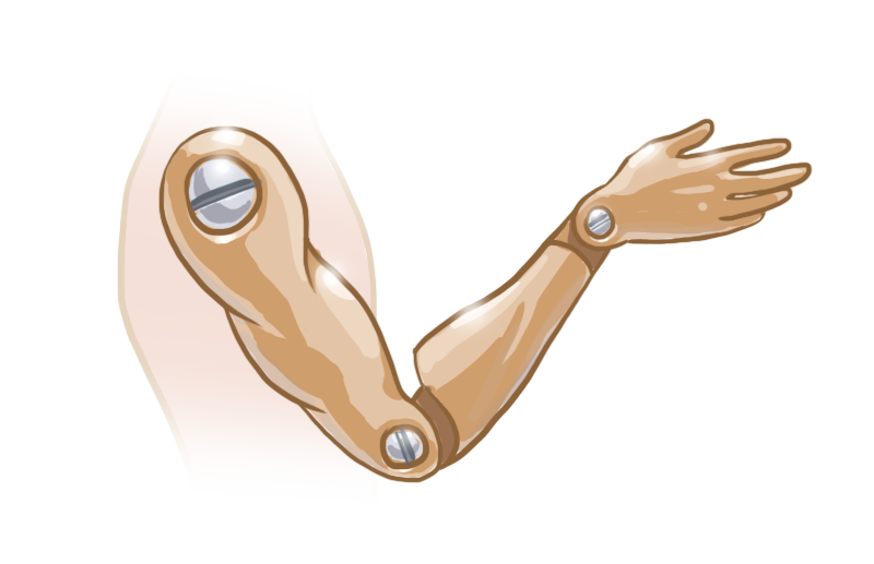
In other words, we have only described unconstrained simulations. The final step to simulating realistic, solid objects, is to apply constraints, defining restrictions on the motion of rigid bodies. Some examples of constraints are joints (such as ball joints and hinge joints), and non-penetration constraints. This last type is what is used to solve collisions, by enforcing behavior that prevents bodies from interpenetrating, and instead causes them to rebound off of each other in a realistic way.
In this article, we’ll discuss equality constraints and inequality constraints within video game physics. We’ll describe them first in terms of a force-based approach, where corrective forces are computed, and then in terms of an impulse-based approach, where corrective velocities are computed instead. Finally, we’ll go over some clever tricks to eliminate unnecessary work and speed up computation.
This installment will involve more heavy-duty math than either Part I or Part II, so be warned. If you need to brush up on your calculus, go here on Khan Academy. For a review of the fundamentals of linear algebra, you can refer to the appendix in Part I, and for the more complex linear algebra, such as matrix multiplication, Khan Academy again delivers. Wikipedia also has great articles on calculus and linear algebra.
What are Constraints?
Constraints are essentially rules that must be satisfied during the simulation, such as “the distance between these two particles should not be greater than 2” or “these two points on this pair of rigid bodies should coincide at all times”. In other words, a constraint removes degrees of freedom from a rigid body. On each step of the simulation, we can compute corrective forces or impulses that, when applied on the bodies, will pull them together or push them apart, so their movement will be restricted and the rules imposed by the constraints will remain satisfied.
In practice, a constraint is defined in terms of a behavior function or constraint function C, which takes the state of a pair of bodies as parameters (e.g. position and orientation) and outputs a scalar number. When the value of this function is in the acceptable range, the constraint is satisfied. Thus, in each step of the simulation, we must apply forces or impulses on the rigid bodies to attempt to keep the value of C in the allowed range.
An Example: Equality Constraints
A common class of constraint is known as an equality constraint. An equality constraint is one in which the only acceptable value of C is zero. Thus, during each step of the simulation, we want to keep C as close to zero as possible. In other words, we want to minimize C. Equality constraints are used when the position of some particle or point must always exactly match some predefined condition. A good example is a ball joint, where two rigid bodies must always be connected at the location of the joint.
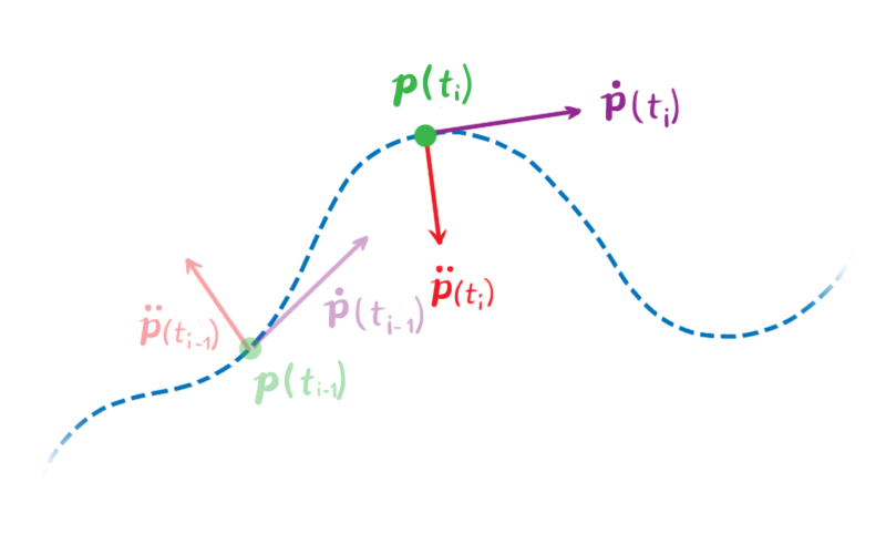
Let’s look at a simple example. Consider a particle in two dimensions, with position p(t) = (px(t), py(t)), which is a function of time that gives the particle’s position at a time t. We’ll use dot notation to express time derivatives, thus, ṗ is the first time derivative of p with respect to time, which is the particle’s velocity v(t), and p̈ is its second time derivative, or it’s acceleration.
Let’s define a constraint. Let C be the following behavior function:

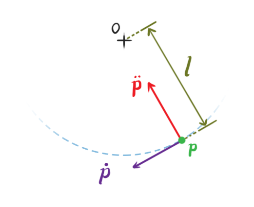
This function takes the particle position as parameter, and outputs its distance from the origin minus l. It will be zero whenever the distance between the particle and the origin is l. Thus the effect of this constraint is to keep the particle at a fixed distance l from the origin, like a pendulum attached to the origin. The values of p that satisfy C(p) = 0 are the legal positions of the particle.
In this example, C is a function of only two variables that outputs a scalar, so we can easily plot it and examine some of its properties. If we set the constraint distance as 2 (that is, l = 2), then the graph of C looks like this:
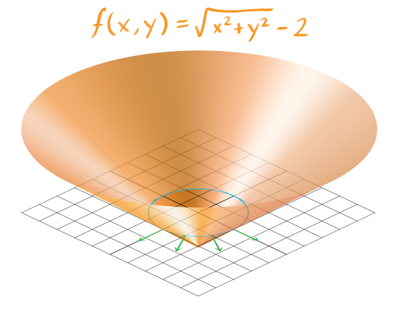
It’s an upside down cone. The blue ring contains the points where C = 0, which are the roots of C. This set of points is known as the constraint hypersurface, and it contains all of the legal positions of our particle. The constraint hypersurface is an s-dimensional surface, where s is the number of variables of C.
The green arrows show gradients of C, evaluated around the hypersurface, and indicates the directions to illegal positions of our particle, where C ≠ 0. If the particle moves in along these lines in any way, either in the positive direction (away from the origin) or the negative direction (towards the origin), it will break the constraint. Thus, the forces we generate to push the particle into legal positions will be parallel to these lines.
While this simple example has only two variables, most constraint functions have more, and that makes it hard to picture what they look like. But the principle remains the same. At each step, we must generate constraint forces that are parallel to the gradient of C at the hypersurface.
Computing Constraint Forces
It would be nice to simply set p such that C is always exactly zero. In practice, this will result in unrealistic behavior, as our particle will jump and jitter around the hypersurface. To keep C as close as possible to zero while maintaining a realistic behavior, an intuitive approach is to use force-based dynamics, and compute the necessary force to apply to the particle so that it will satisfy the constraints without breaking Newton’s laws of motion.
To compute the constraint force, we will need to have a grasp of the allowable accelerations and velocities of the particle. To this end, we must obtain the derivatives of C with respect to time.
We want to ensure that the value of C will stay equal to zero, and remain unchanged throughout the simulation. This means that the first time derivative, Ċ, must be zero as well.
Likewise, in order for Ċ to remain fixed at zero, the second derivative, C̈, must also be zero.
We do not have to constrain any further derivatives of C, because the second derivative is where our constraint forces will be applied.
Let’s determine these derivatives. Our current definition of C has a square root in it, and that makes differentiation a bit difficult. We can rewrite C though, using squared distances:

This doesn’t change the property that C will be zero when the distance between the particle and the origin is l. From this, we can get the first derivative of C with respect to t:

Given a legal position of p, all velocities ṗ that satisfy Ċ(p) = 0 are legal velocities. In this example, these should be only those velocities that are tangential to the hypersurface in the above image.
The second derivative of C with respect to t is:

Equivalently, given a legal position and velocity, all accelerations p̈ that satisfy C̈(p) = 0 are legal accelerations. In this example, these should be only those accelerations that are directly towards or away from the origin.
Using Newton’s Second Law of motion we can express the acceleration in terms of force. We can consider that there are two forces acting on the particle: a combination of all external forces fext, such as gravity, wind, and forces applied by the user, and the constraint force fC. The latter is the one we want to determine. Assuming the particle has mass m, its acceleration is:

Substituting this into C̈ = 0 we get:

Which can be rearranged to:

We have a single equation and two unknowns (the two coordinates of fC), thus it cannot be solved. We need to introduce one additional condition.
Intuitively, we know that the constraint force must be applied to oppose to the direction we want to prevent the particle from moving in. In this example, the constraint forces will always point to a direction that is perpendicular to the circle of radius l, because the particle is not allowed to move outside this circle. These perpendicular forces will push the particle back into the circular path whenever it tries to leave it, and this causes the velocity component that points in these directions to be zero. Thus, the constraint forces be always perpendicular to the velocity of the particle.
Therefore:

The equation for the first derivative of our constraint says that p · ṗ = 0. Since fC · ṗ = 0, we have that both fC and p are orthogonal to ṗ, and so fC and p are parallel. Thus, we can write one as a multiple of the other

We are nearly there! The scalar λ represents the magnitude of the constraint force that should be applied to bring the system to a valid state. The further our system moves away from the valid states, the bigger λ will be in order to push it back to a valid state. At this point λ is our only unknown. Substituting the above into our previous equation we obtain:

Now we can compute λ directly and obtain fC by multiplying it with p. Then we simply apply fC to the particle, and let the simulation described in Part I do the rest!
λ is also known as a Lagrange multiplier. For any constraint, the calculation involves determining the direction of the force vector, and it’s magnitude, λ.
When to Apply Constraint Forces
From this example, we can see that computing the constraint forces requires that all other forces fext are already known. And of course, we must apply the constraint forces before simulating the resulting motion. Thus, a generalized sequence for each simulation step look like this:
- Compute all external forces fext.
- Compute the constraint forces fC.
- Apply all the forces and simulate the motion, as described in Part I.
Systems of Constraints
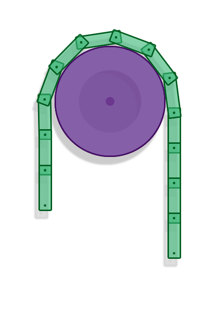
That was a relatively simple example of a pretty basic constraint involving one single entity. We actually want to be able to have many constraints and many objects in our simulation. Constraints cannot be handled in isolation because the forces applied by one constraint might influence the forces that are applied by another constraint. That is clearly visible in the example of a chain of rigid bodies connected by revolute joints. For that reason, constraints must be solved as a whole, in a system of equations.
Setting Up
We’ll now work with vectors and matrices that contain the state of all entities in our simulation, and use them to develop our global equations in a similar manner to what we did for the single particle example. Let’s develop these equations for rigid bodies in two dimensions.
State Vector
Say we have n rigid bodies we are simulating. Let q be a state vector that has all the rigid bodies’ positions and angles:
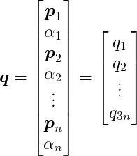
where pi is a two-dimensional vector representing the position of the i-th rigid body, and αi is its angle, which is a scalar. Thus, q has 3n elements.
Dynamics: Newton’s Second Law
Let M be the following 3n by 3n diagonal matrix:
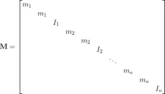
where mi is the mass of the i-th rigid body, and Ii is its moment of inertia.
Let F be a global force vector that contains the forces and torques acting on each body. It’s the sum of external and constraint forces:

and:
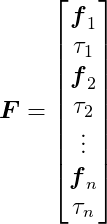
F also has 3n elements, since each fi is a vector of two dimensions.
Now we can write Newton’s Second Law of motion for the whole set of bodies with one expression:

Constraints
Finally, let’s set up our behavior functions. Say there are m constraints, each representing a link in the chain of rigid bodies. We are going to group all our behavior functions into a single function C(q):
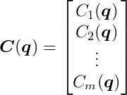
C(q) takes the 3n-dimensional vector q as input, and outputs an m-dimensional vector. We want to keep this output as close to the zero vector as possible, using a similar process to what we did above.
We aren’t going to get into defining each behavior function here, as it won’t be necessary, but the web has great tutorials on revolute joint constraints.
Derivatives of C Over Time
As before, we also want the first and second time derivatives of C to be zero vectors. Let’s develop these equations.
The derivative of C with respect to time can be given as:

Note the use of the chain rule. We can develop this equation further, by defining J as:

This is the Jacobian Matrix, or the Jacobian of C. The Jacobian is a generalization of the gradient, which is itself a generalization of the slope. It’s also interesting to note that each row is the gradient of each behavior function. The Jacobian tells us how every behavior function reacts to changes with respect to every state variable.
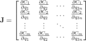
In the case of our chain, it will be a sparse matrix, because each constraint only involves the two rigid bodies linked by that constraint. The state of all other bodies will have no direct effect on that link.
We can now express the time derivative of C as:

Beautiful.
The second derivative of C will be:

where:

Substituting our expression of Newton’s Second Law we have:

Computing the Constraint Force Vector
We want the second derivative of C to be zero, so let’s set it to zero and rearrange:

This equation is analogous to the one we developed before for a single constraint:

Again, the number of unknowns is greater than the number of equations, and again, we can use the fact that constraint forces are orthogonal to the velocities to find a solution:

We also want the first derivative of C to be zero. From Ċ = 0 we have that:

and therefore we can write the constraint force vector FC as a multiple of J:

The vector λ has m scalar components, and in this matrix-vector multiplication, each component λi multiplies a row of J (which is the gradient of the i-th constraint function) and sums them together. That is

FC is thus a linear combination of the rows of J, which are the gradients of the constraint functions. Although this system is too complex to be able to easily visualize the hypersurface, as we did for the particle example, it behaves just the same as that example: the gradients are orthogonal to the constraints’ hypersurfaces, and are the directions in which the system is not allowed to move. Hence, this is a linear combination of vectors that point in the prohibited directions, meaning that the constraint forces will be restricted to these directions and they will push the bodies towards the valid states imposed by the constraints.
The only thing remaining to solve for is the λ vector, which will determine the magnitudes of the constraint forces. Let’s get back to our main equation and substitute the last expression in there:

This is a system of linear equations where only λ is not known. There are plenty of well known methods to solve a linear system like this efficiently. Once it’s solved and we have λ, we can compute FC, apply the results to the rigid bodies, and simulate the resulting motion as shown in Part I.
For a detailed derivation of these equations check out Andrew Witkin’s Constrained Dynamics, part of the Physically Based Modeling: Principles and Practice course at Carnegie Mellon University.
Inequality Constraints
Up to now, we have assumed that our behavior functions must be equal to zero at all times for the constraints to be satisfied. There are, however, types of constraints that require some flexibility, where corrective forces won’t be applied for a wider range of values of C than just zero. An example of one such constraint is the non-penetration constraint, which is often the most important type of constraint in rigid body simulations, because it is responsible for collision resolution, ensuring two bodies never interpenetrate unrealistically, and giving them a natural solid behavior.
As we described in Part II, after a collision is detected by the GJK algorithm, we’ll have the contact points on both bodies as well as the a surface normal at the contact point. Remember that GJK is both a collision test and a proximity test, and that two bodies may be considered “colliding” even if they are not actually touching, but the distance between them is very small. In this case, the contact points on the two bodies are considered to be the points where they are closest to each other.
The non-penetration constraint will strive to keep the bodies separated by applying corrective forces that push the bodies apart, but only if the bodies are colliding.
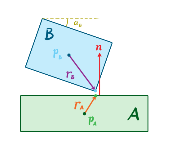
Consider a pair of 2-dimensional bodies A and B that are colliding. At the moment of contact, A has position pA and angle αA, and B has position pB and angle αB. Let’s call rA a vector that goes from the center of A to the contact point on A, and let’s also define rB similarly. Let n be the contact normal that points from A to B.
Let’s take a standard 2D rotation matrix R(θ) that rotates vectors by a given angle θ:

We can use it to rotate the vectors rA and rB by the angles αA and αB, respectively. This allows us to define a behavior function, C, as:

This behavior function looks daunting, but it’s action is simple. It takes a vector between the contact point on A and the contact point on B, projects it onto the normal vector n, and outputs the length of this projection vector. In other words, it determines the penetration depth in the direction of the normal. If C is greater than or equal to zero, no force should be applied, because the bodies are not penetrating. Thus, we need to enforce the inequality C ≥ 0.
If we analyze the equations, we’ll find we need only to restrict the value of λ for each constraint. In the equality constraints of the previous examples, λ can take any value, meaning the constraint forces could be in either a positive or negative direction along the behavior gradients). In an inequality constraint such as the non-penetration constraint, however, λ must be greater than or equal to zero, which represents constraint forces that can only push away the colliding bodies away from each other.
This change transforms the system of linear equations we have into something quite different (and more complicated) called a Mixed Linear Complementarity Problem, or MLCP. There are a few nice algorithms that can solve this problem directly, such as Lemke’s Algorithm. However, we’ll skip the details here, and discuss another approach to constraints that is very popular in game physics.
Impulse-Based Dynamics
So far, we have examined the force-based approach to enforcing constraints. We calculate the constraint forces, apply these forces on the bodies together with the external forces, and integrate them using the methods we described in Part I to simulate the resulting motions. There is, however, another technique that is very popular among game physics engines, which takes an impulse-based approach, operating on the velocity of the bodies and not on the force or acceleration. This means the constraint solver calculates and applies a direct change in the linear and angular velocities of the bodies, instead of calculating and applying corrective forces and relying on integration to then change the velocities.
With impulse-based dynamics, the goal is to find the impulses that result in velocities that solve the constraints. This is somewhat analogous to the force-based goal of finding the forces that will result in accelerations that solve the constraints. However, we are working at a lower order of magnitude, and as a result, the math is less complex.
The impulse-based approach was popularized by Brian Mirtich in his PhD thesis from 1996, which is still one of the most important references on the topic. Jan Bender et. al. have also published a series of important papers on the subject.
The general sequence of a simulation step using impulse-based dynamics is somewhat different from that of force-based engines:
- Compute all external forces.
- Apply the forces and determine the resulting velocities, using the techniques from Part I.
- Calculate the constraint velocities based on the behavior functions.
- Apply the constraint velocities and simulate the resulting motion.
Perhaps the biggest advantage of impulse-based dynamics over the force-based approach and others is the relative simplicity of the algorithms. It is also easier to understand intuitively. In most cases, it is also more computationally efficient, which makes it more appealing for games, where real-time performance is often a priority. There are drawbacks to take into account, however, including difficulty realistically handling stable contacts (like in a resting stack of boxes), and added complexity when modeling contact friction. Nevertheless, we can work around these issues in a couple of ways, as we’ll see further down.
In physics parlance, an impulse is the integral of a force with respect to time. That is:

This is equal to the change in momentum during that time.
If a constant force F is applied for an amount of time h, then the impulse is simply:

When two rigid objects collide, they stay in contact for a very short amount of time, during which they deform and apply equal and opposite forces on each other. After this brief interaction, their velocities may have changed drastically, and therefore so might their momentums. If the objects are perfectly rigid bodies, the amount of time they stay in contact is infinitesimally close to zero, and their velocities change immediately after a collision. Perfectly rigid bodies do not exist in real life, but the simplification can be used to realistically simulate the behavior of objects that are very rigid.
Sequential Impulses
Our goal is to find the impulses that solve the constraints for the current time step of the simulation. Sequential impulses is a technique we can use to find these impulses. It was popularized by Erin Catto, the author of the Box2D physics engine. It is an iterative algorithm, where the idea is to hone in on the constraint velocity by applying impulses on the rigid bodies on each iteration, and repeat until resulting velocity error is very small, or in other words, until Ċ is very close to zero.
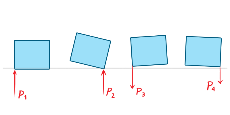
In sequential impulses, we don’t create one monolithic system of equations and inequalities like we did before. We actually model and solve each constraint individually, pretty much like we did in the first example for one particle. The algorithm boils down to these three steps:
-
Integrate applied forces using semi-implicit Euler as in Part I, yielding tentative velocities. These velocities may violate the constraints and need to be corrected before being applied.
-
Apply impulses sequentially for all constraints, to correct the velocity errors. Repeat for several iterations, until impulses become small or after a maximum number of iterations is reached.
-
Use the new velocities to simulate motion, updating positions, again using semi-implicit Euler.
Note that these steps correspond to steps 2 through 4 of the general sequence of impulse-based time steps described above.
Computing the Velocities
Let’s examine the equations. Let q̇1 = q̇(ti-1) and q̇2 = q̇(ti). That is, q̇1 and q̇2 are the velocity in the previous time step and the velocity for the current time step (which we want to determine), respectively. Using the semi-implicit Euler integration scheme, the tentative, unconstrained velocity for the current step (indicated by an asterisk) is:

This velocity may violate the constraints, in which case it must be corrected with an impulse.
Let PC be the constraint impulse. Dividing it by mass we get the change in velocity, and apply it to the tentative velocity to get the desired velocity that satisfies the constraints:

So how do we determine PC? If we recognize that the impulse will be applied in the same direction as an instantaneous force that produces it, we can again use the fact that the constraint forces must be parallel to the gradient of the behavior function, just like we did with the force-based constraints. Thus, we can write:

where λ is again a vector of magnitudes.
The impulse-based approach represents a shortcut that bypasses Newton’s Second Law. By skipping the computation of forces and their resulting accelerations, it can generate noticeable, instantaneous velocity changes that can make a simulation jitter undesirably. To mitigate these effects, it’s common to add a bias factor to the velocity constraints, to soften the effects:

Observe that Jq̇2 + b = 0, since q̇2 must be a valid velocity. Then, substituting and rearranging the valid velocity equation, we obtain

After solving this equation for λ we can compute the constraint impulse using PC = JTλ, and finally update the velocity.
We have to solve every constraint individually and apply the impulses, updating the bodies’ velocities, and then repeat this step multiple times until convergence is achieved or a maximum number of iterations is met. That means we accumulate the impulses as we iterate. To finish the time step, we just have to update the positions using the final velocities:

Inequality Constraints
For inequality constraints, we have to bound the impulses and keep them in the allowable values as we accumulate them, so that the constraints won’t apply impulses in undesired directions or strengths. This bounding procedure is not as simple as just applying a min/max function, because we only want to bound the final accumulated impulse, but not the intermediate impulses generated during the accumulation. Check out Erin Catto’s GDC 2009 presentation for details.
Warm Starting
One little technique that improves the accuracy of the algorithm greatly is called warm starting. The algorithm starts with an initial guess for λ, and works its way up from there. Given that a physics simulation has a lot of temporal and spatial coherence, it’s natural to think about using the λ found in the previous step as a starting point, and that is what warm starting is about. The bodies often don’t move much from step to step, so it’s very likely that the impulses we computed in the previous step will be almost the same in the current step. Starting our algorithm from there makes it converge to a more accurate solution faster. This improves the stability of the simulation, especially for constraints such as joints and persistent contact between bodies.
Projected Gauss-Seidel
Another technique for solving impulse-based constraints comes from the fact that it can also be modeled as an MLCP. Projected Gauss-Seidel (PGS) is an iterative algorithm for solving MLCPs that works well for impulse-based dynamics. It essentially solves a linear system Ax = b, with bounds on x. PGS is an extension of the Gauss-Seidel method, where we bound the value of x on each iteration to keep it in the desired range.
Since we’re working on the velocity, we can eliminate the acceleration by writing an approximation of it as the ratio between the velocity change and the delta time for the current time step. Let q̇1 = q̇(ti-1) and q̇2 = q̇(ti), then:

where, again, q̇1 is the velocity calculated in the previous step, and q̇2 is the velocity we want to find for the current step. From Newton’s Second Law we have:

Substituting our approximation and FC = JTλ, we get:

Since Ċ = 0, we have that Jq̇2 = 0, because q̇2 will be a legal velocity after this is solved. Rearranging and multiplying by J on both sides, we get:

This MLCP is slightly different from what we have for the force-based approach, because it uses an approximate acceleration. Once we solve it using PGS, we’ll have λ, and then q̇2 can be computed using the previous equation:

The updated positions and orientations follow easily from the semi-implicit Euler scheme:

Interestingly, close investigation reveals that PGS is equivalent to sequential impulses! We’re doing essentially the same thing here. Warm starting can again be used, taking λ computed in the previous step as a starting point. The difference is that the sequential impulses formulation is more intuitive, but the PGS formulation is more general and allows for more flexible code. For instance, we can experiment using other tools to solve the MLCP.
For more details about using PGS in an impulse-based simulation, take a look at Erin Catto’s 2005 GDC presentation and paper.
Simulating Friction Using Impulses
The Coulomb friction model is simple and works nicely. It defines two different cases when two solid surfaces are in contact with each other:
- Static friction: Resistance to tangential motion when the surfaces are not moving relative to each other, because there is not enough force to overcome friction. The friction force points in the opposite direction of the net tangent force, and is equal to it in magnitude.
- Kinetic friction: Resistance to tangential motion when the surfaces are sliding. The friction force points in the opposite direction of motion, and is less than the net tangent forces in magnitude.
The friction force is proportional to the normal force, which is the net force component in the direction of the contact surface’s normal vector. In other words, the force of friction is proportional to the force pushing the two objects towards into each other. It can be expressed by:

where Ff is the friction force, Fn is the normal force and μ is the coefficient of friction (which can be different for static and kinetic friction).
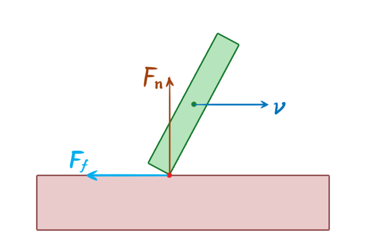
To simulate friction using a constraint model, we have to write a velocity constraint directly:

Where vp is the relative velocity vector at the contact point p, and t is a unit vector tangent to the surfaces. We want to bring the tangential velocity to zero.
Per the friction equation, we have to limit the value of the friction impulse to the normal impulse times the coefficient of friction. This means we have to keep our λ between -μ λn and μ λn, where λn is the magnitude of the normal impulse.

Thus, friction is another example of an inequality constraint.
In three dimensions, things get a tad more complicated. In his 2005 GDC presentation, Erin Catto presents an approach that uses two tangent vectors and a pair of constraints. However, limiting the friction impulse by a multiple of the normal impulse in this case couples the two constraints, and makes things hard to solve. He works around that by instead limiting it it by a constant value proportional to the mass of the body and the gravity acceleration.
Optimizations
We’ve described several methods for determining either the forces or the impulses to apply to our rigid bodies in order to enforce our constraints. In each case, the calculations involve a good amount of legwork. Let’s now look at some clever optimization strategies to cut out some of this work when it isn’t necessary.
Islands
In a constrained physics simulation, one can observe that some objects influence the motion of others, while some don’t.
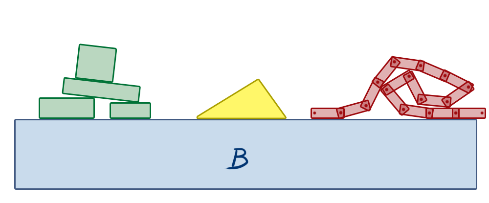
In the above image, the box B is a static object that doesn’t move. It’s the floor. The objects on the left are stacked, in contact with each other. If any of them move at all, the others will potentially move as well, because there are contact constraints between them. Any force or impulse that is applied to any of these bodies might propagate throughout the other bodies. However, the triangle in the middle is just sitting alone on the fixed box B. Forces applied on the stacked objects on the left will never affect the motion of the triangle, because there’s no connection between any of the stacked objects and the triangle. The same can be said about the chain of boxes on the right. They’re all connected by revolute joints, and so the motion of any of them can generate a reaction along the constraints, influencing the motion of all other boxes that are part of the chain. But they will never influence the state of the triangle, nor the stacked objects on the left, unless a new constraint is created between any of these, such as a contact/non-penetration constraint due to their motion causing them to collide with the other objects.
Based on this simple observation, we can group these objects into what we call islands, which are self contained groups of bodies that can influence the motion of each other in the group through constraint forces/impulses, but will not influence the movement of objects belonging to any other island.
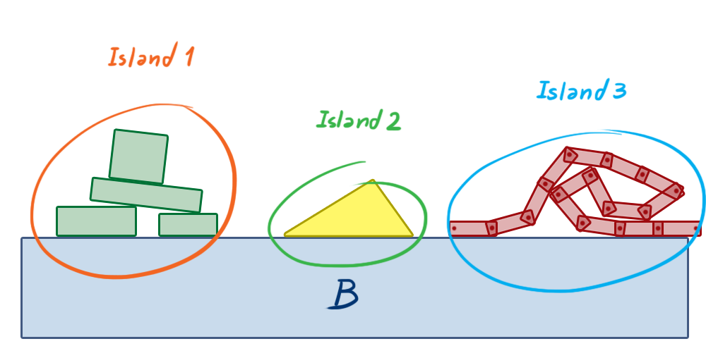
This separation allows us to solve smaller groups of constraints, creating smaller systems instead of one single big system for the whole physics world. This eliminates a potentially huge amount of useless work that the computer must perform.
If we look at the world as a graph, where bodies are nodes and constraints are edges, we can build the islands using a depth-first search on this graph. In graph theory, our islands are known as connected components.
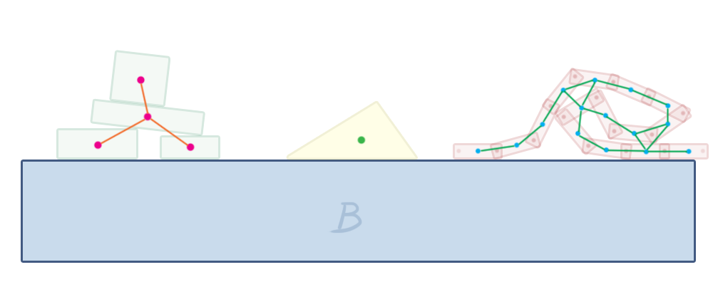
Box2D does this in its b2World::Solve method, which is responsible for solving all the constraints in each step. It builds the islands and then calls b2Island::Solve on each of them. This method solves the constraints in that island using sequential impulses.
Sleeping
When a body comes to rest during the simulation, its position will naturally remain unchanged for all subsequent steps of the simulation, until some external force causes it to move again. This calls our attention to another possible optimization: we can stop simulating a given island when the linear and angular velocities of all its bodies stay below a given tolerance for a small amount of time. This condition is called sleeping.
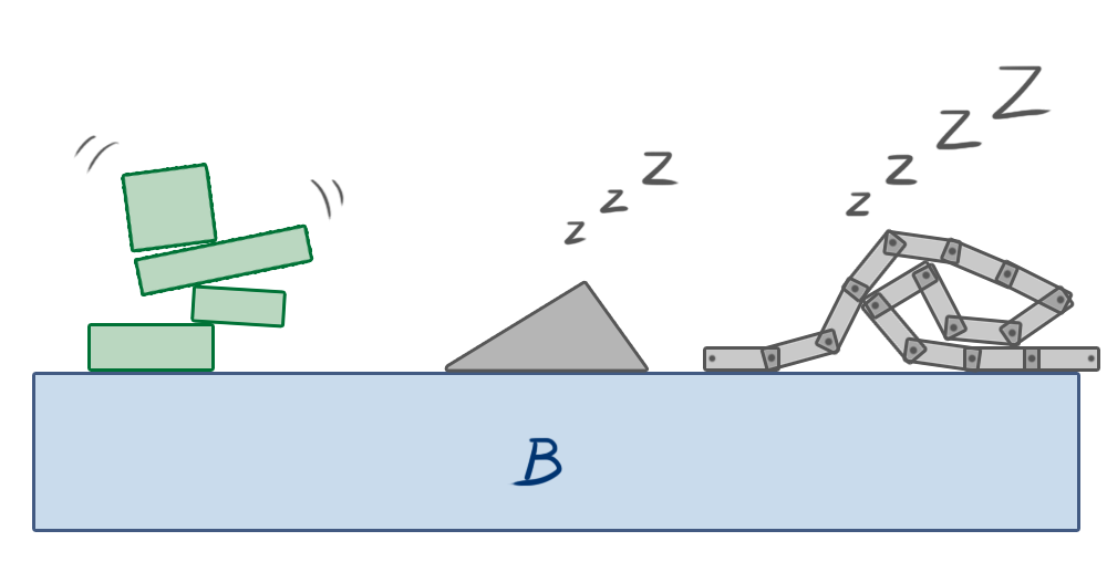
After an island is put to sleep, its bodies are excluded from all steps of the simulation except collision detection. If a body outside the island collides with any body of this island, the island “wakes up,” and gets back into the simulation again. If any other external force or impulse is applied on any of its bodies, it also wakes up.
This is a rather simple technique that can greatly improve the performance of simulations containing many objects.
Conclusion - Video Game Physics and Constrained Rigid Body Simulation
This concludes our three-part series on video game physics. We have seen how physics can be simulated in games, focusing on rigid body simulation, which is a foundational subset of physics simulation that is often enough to make games dynamic and fun. We saw how the motion of rigid bodies can be simulated, how collisions between them can be detected and solved, and also how other interactions among them can be modeled.
The techniques we’ve seen are used in popular game physics engines such as Box2D, Chipmunk Physics and Bullet Physics. These methods can be used to make games with realistic, dynamic behavior, with objects moving around and colliding, and also allows objects to be connected to one another in a variety of ways through joints of many types. It may be of interest to note that these same methods even find applications in other realms beyond gaming, such as robotics.
As usual, things may be beautiful in theory, but in practice turn out to be another story. Many clever simplifications are necessary to obtain a stable and efficient implementation, especially regarding constrained dynamics. Many great developments have been made over the last few years regarding collision detection, time of impact computation, MLCP resolution, and so on, and yet there are still many things that can be improved. The Bullet Physics Forum is a good place to keep up to date on what is going on in the game and rigid body physics simulation world, particularly the Research and development discussion about Collision Detection and Physics Simulation section, where members discuss modern physics simulation techniques of all sorts.

Further Reading on the Toptal Blog:
Bella Vista, Panama City, Panama, Panama
Member since February 19, 2013
About the author
Nilson (dual BCS/BScTech) been an iOS dev and 2D/3D artist for 8+ years, focusing on physics and vehicle simulations, games, and graphics.

