3D Graphics: A WebGL Tutorial
Whether you just want to create an interactive 3D logo, on the screen or design a fully fledged game, knowing the principles of 3D graphics rendering will help you achieve your goal.
In this article, Toptal Freelance Software Engineer Adnan Ademovic gives us a step-by-step tutorial to rendering objects with textures and lighting, by breaking down abstract concepts like objects, lights, and cameras into simple WebGL procedures.
Adnan has experience in desktop, embedded, and distributed systems. He has worked extensively in C++, Python, and in other languages.
Expertise
The world of 3D graphics can be very intimidating to get into. Whether you just want to create an interactive 3D logo, or design a fully fledged game, if you don’t know the principles of 3D rendering, you’re stuck using a library that abstracts out a lot of things.
Using a library can be just the right tool, and JavaScript has an amazing open source one in the form of three.js. There are some disadvantages to using pre-made solutions, though:
- They can have many features that you don’t plan to use. The size of the minified base three.js features is around 500kB, and any extra features (loading actual model files is one of them) make the payload even larger. Transferring that much data just to show a spinning logo on your website would be a waste.
- An extra layer of abstraction can make otherwise easy modifications hard to do. Your creative way of shading an object on the screen can either be straightforward to implement or require tens of hours of work to incorporate into the library’s abstractions.
- While the library is optimized very well in most scenarios, a lot of bells and whistles can be cut out for your use case. The renderer can cause certain procedures to run millions of times on the graphics card. Every instruction removed from such a procedure means that a weaker graphics card can handle your content without problems.
Even if you decide to use a high-level graphics library, having basic knowledge of the things under the hood allows you to use it more effectively. Libraries can also have advanced features, like ShaderMaterial in three.js. Knowing the principles of graphics rendering allows you to use such features.
Our goal is to give a short introduction to all the key concepts behind rendering 3D graphics and using WebGL to implement them. You will see the most common thing that is done, which is showing and moving 3D objects in an empty space.
The final code is available for you to fork and play around with.
Representing 3D Models
The first thing you would need to understand is how 3D models are represented. A model is made of a mesh of triangles. Each triangle is represented by three vertices, for each of the corners of the triangle. There are three most common properties attached to vertices.
Vertex Position
Position is the most intuitive property of a vertex. It is the position in 3D space, represented by a 3D vector of coordinates. If you know the exact coordinates of three points in space, you would have all the information you need to draw a simple triangle between them. To make models look actually good when rendered, there are a couple more things that need to be provided to the renderer.
Vertex Normal
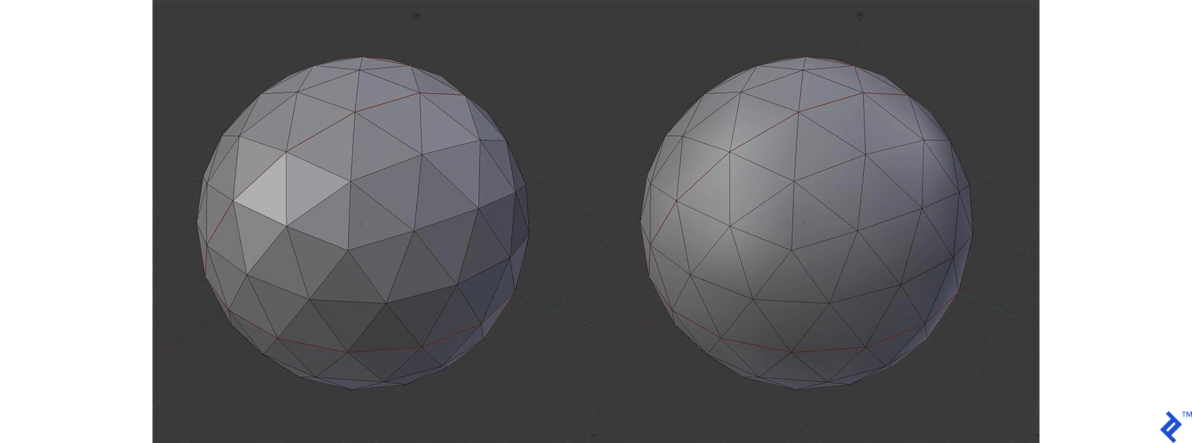
Consider the two models above. They consist of the same vertex positions, yet look totally different when rendered. How is that possible?
Besides telling the renderer where we want a vertex to be located, we can also give it a hint on how the surface is slanted in that exact position. The hint is in the form of the normal of the surface at that specific point on the model, represented with a 3D vector. The following image should give you a more descriptive look at how that is handled.
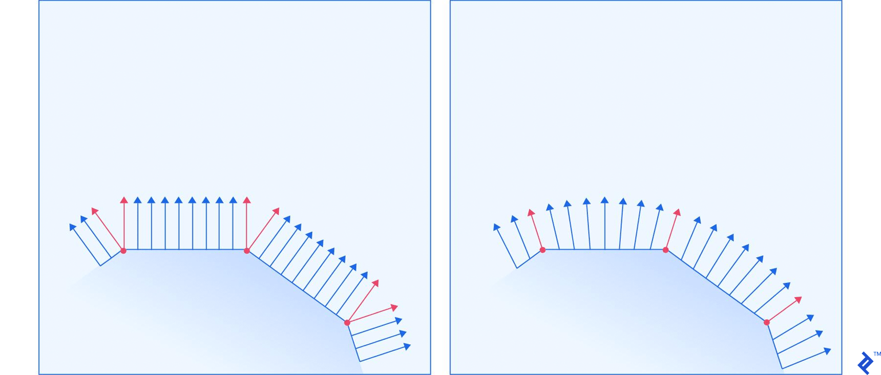
The left and right surface correspond to the left and right ball in the previous image, respectively. The red arrows represent normals that are specified for a vertex, while the blue arrows represent the renderer’s calculations of how the normal should look for all the points between the vertices. The image shows a demonstration for 2D space, but the same principle applies in 3D.
The normal is a hint for how lights will illuminate the surface. The closer a light ray’s direction is to the normal, the brighter the point is. Having gradual changes in the normal direction causes light gradients, while having abrupt changes with no changes in-between causes surfaces with constant illumination across them, and sudden changes in illumination between them.
Texture Coordinates
The last significant property are texture coordinates, commonly referred to as UV mapping. You have a model, and a texture that you want to apply to it. The texture has various areas on it, representing images that we want to apply to different parts of the model. There has to be a way to mark which triangle should be represented with which part of the texture. That’s where texture mapping comes in.
For each vertex, we mark two coordinates, U and V. These coordinates represent a position on the texture, with U representing the horizontal axis, and V the vertical axis. The values aren’t in pixels, but a percentage position within the image. The bottom-left corner of the image is represented with two zeros, while the top-right is represented with two ones.
A triangle is just painted by taking the UV coordinates of each vertex in the triangle, and applying the image that is captured between those coordinates on the texture.
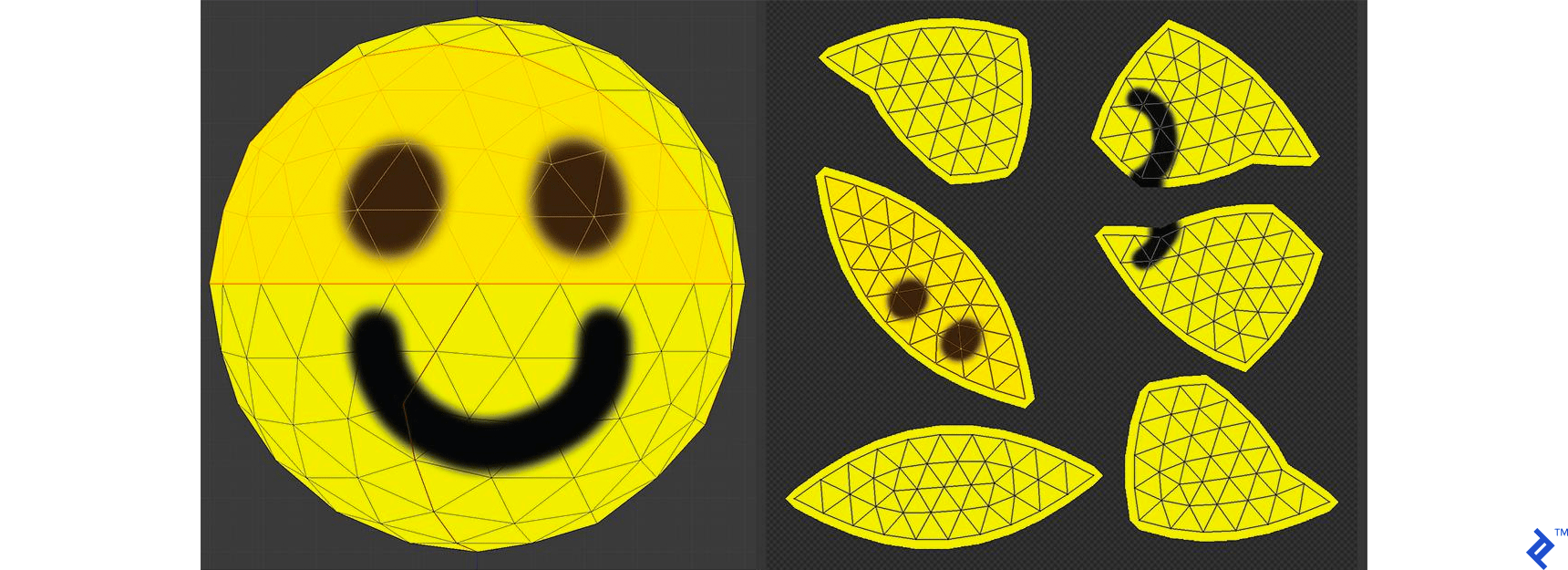
You can see a demonstration of UV mapping on the image above. The spherical model was taken, and cut into parts that are small enough to be flattened onto a 2D surface. The seams where the cuts were made are marked with thicker lines. One of the patches has been highlighted, so you can nicely see how things match. You can also see how a seam through the middle of the smile places parts of the mouth into two different patches.
The wireframes aren’t part of the texture, but just overlayed over the image so you can see how things map together.
Loading an OBJ Model
Believe it or not, this is all you need to know to create your own simple model loader. The OBJ file format is simple enough to implement a parser in a few lines of code.
The file lists vertex positions in a v <float> <float> <float> format, with an optional fourth float, which we will ignore, to keep things simple. Vertex normals are represented similarly with vn <float> <float> <float>. Finally, texture coordinates are represented with vt <float> <float>, with an optional third float which we shall ignore. In all three cases, the floats represent the respective coordinates. These three properties are accumulated in three arrays.
Faces are represented with groups of vertices. Each vertex is represented with the index of each of the properties, whereby indices start at 1. There are various ways this is represented, but we will stick to the f v1/vt1/vn1 v2/vt2/vn2 v3/vt3/vn3 format, requiring all three properties to be provided, and limiting the number of vertices per face to three. All of these limitations are being done to keep the loader as simple as possible, since all other options require some extra trivial processing before they are in a format that WebGL likes.
We’ve put in a lot of requirements for our file loader. That may sound limiting, but 3D modeling applications tend to give you the ability to set those limitations when exporting a model as an OBJ file.
The following code parses a string representing an OBJ file, and creates a model in the form of an array of faces.
function Geometry (faces) {
  this.faces = faces || []
}

// Parses an OBJ file, passed as a string
Geometry.parseOBJ = function (src) {
  var POSITION = /^v\s+([\d\.\+\-eE]+)\s+([\d\.\+\-eE]+)\s+([\d\.\+\-eE]+)/
  var NORMAL = /^vn\s+([\d\.\+\-eE]+)\s+([\d\.\+\-eE]+)\s+([\d\.\+\-eE]+)/
  var UV = /^vt\s+([\d\.\+\-eE]+)\s+([\d\.\+\-eE]+)/
  var FACE = /^f\s+(-?\d+)\/(-?\d+)\/(-?\d+)\s+(-?\d+)\/(-?\d+)\/(-?\d+)\s+(-?\d+)\/(-?\d+)\/(-?\d+)(?:\s+(-?\d+)\/(-?\d+)\/(-?\d+))?/

  lines = src.split('\n')
  var positions = []
  var uvs = []
  var normals = []
  var faces = []
  lines.forEach(function (line) {
    // Match each line of the file against various RegEx-es
    var result
    if ((result = POSITION.exec(line)) != null) {
      // Add new vertex position
      positions.push(new Vector3(parseFloat(result[1]), parseFloat(result[2]), parseFloat(result[3])))
    } else if ((result = NORMAL.exec(line)) != null) {
      // Add new vertex normal
      normals.push(new Vector3(parseFloat(result[1]), parseFloat(result[2]), parseFloat(result[3])))
    } else if ((result = UV.exec(line)) != null) {
      // Add new texture mapping point
      uvs.push(new Vector2(parseFloat(result[1]), 1 - parseFloat(result[2])))
    } else if ((result = FACE.exec(line)) != null) {
      // Add new face
      var vertices = []
      // Create three vertices from the passed one-indexed indices
      for (var i = 1; i < 10; i += 3) {
        var part = result.slice(i, i + 3)
        var position = positions[parseInt(part[0]) - 1]
        var uv = uvs[parseInt(part[1]) - 1]
        var normal = normals[parseInt(part[2]) - 1]
        vertices.push(new Vertex(position, normal, uv))
      }
      faces.push(new Face(vertices))
    }
  })

  return new Geometry(faces)
}

// Loads an OBJ file from the given URL, and returns it as a promise
Geometry.loadOBJ = function (url) {
  return new Promise(function (resolve) {
    var xhr = new XMLHttpRequest()
    xhr.onreadystatechange = function () {
      if (xhr.readyState == XMLHttpRequest.DONE) {
        resolve(Geometry.parseOBJ(xhr.responseText))
      }
    }
    xhr.open('GET', url, true)
    xhr.send(null)
  })
}

function Face (vertices) {
  this.vertices = vertices || []
}

function Vertex (position, normal, uv) {
  this.position = position || new Vector3()
  this.normal = normal || new Vector3()
  this.uv = uv || new Vector2()
}

function Vector3 (x, y, z) {
  this.x = Number(x) || 0
  this.y = Number(y) || 0
  this.z = Number(z) || 0
}

function Vector2 (x, y) {
  this.x = Number(x) || 0
  this.y = Number(y) || 0
}
The Geometry structure holds the exact data needed to send a model to the graphics card to process. Before you do that though, you’d probably want to have the ability to move the model around on the screen.
Performing Spatial Transformations
All the points in the model we loaded are relative to its coordinate system. If we want to translate, rotate, and scale the model, all we need to do is perform that operation on its coordinate system. Coordinate system A, relative to coordinate system B, is defined by the position of its center as a vector p_ab, and the vector for each of its axes, x_ab, y_ab, and z_ab, representing the direction of that axis. So if a point moves by 10 on the x axis of coordinate system A, then—in the coordinate system B—it will move in the direction of x_ab, multiplied by 10.
All of this information is stored in the following matrix form:
x_ab.x  y_ab.x  z_ab.x  p_ab.x
x_ab.y  y_ab.y  z_ab.y  p_ab.y
x_ab.z  y_ab.z  z_ab.z  p_ab.z
     0       0       0       1
If we want to transform the 3D vector q, we just have to multiply the transformation matrix with the vector:
q.x
q.y
q.z
1
This causes the point to move by q.x along the new x axis, by q.y along the new y axis, and by q.z along the new z axis. Finally it causes the point to move additionally by the p vector, which is the reason why we use a one as the final element of the multiplication.
The big advantage of using these matrices is the fact that if we have multiple transformations to perform on the vertex, we can merge them into one transformation by multiplying their matrices, prior to transforming the vertex itself.
There are various transformations that can be performed, and we’ll take a look at the key ones.
No Transformation
If no transformations happen, then the p vector is a zero vector, the x vector is [1, 0, 0], y is [0, 1, 0], and z is [0, 0, 1]. From now on we’ll refer to these values as the default values for these vectors. Applying these values gives us an identity matrix:
1 0 0 0
0 1 0 0
0 0 1 0
0 0 0 1
This is a good starting point for chaining transformations.
Translation
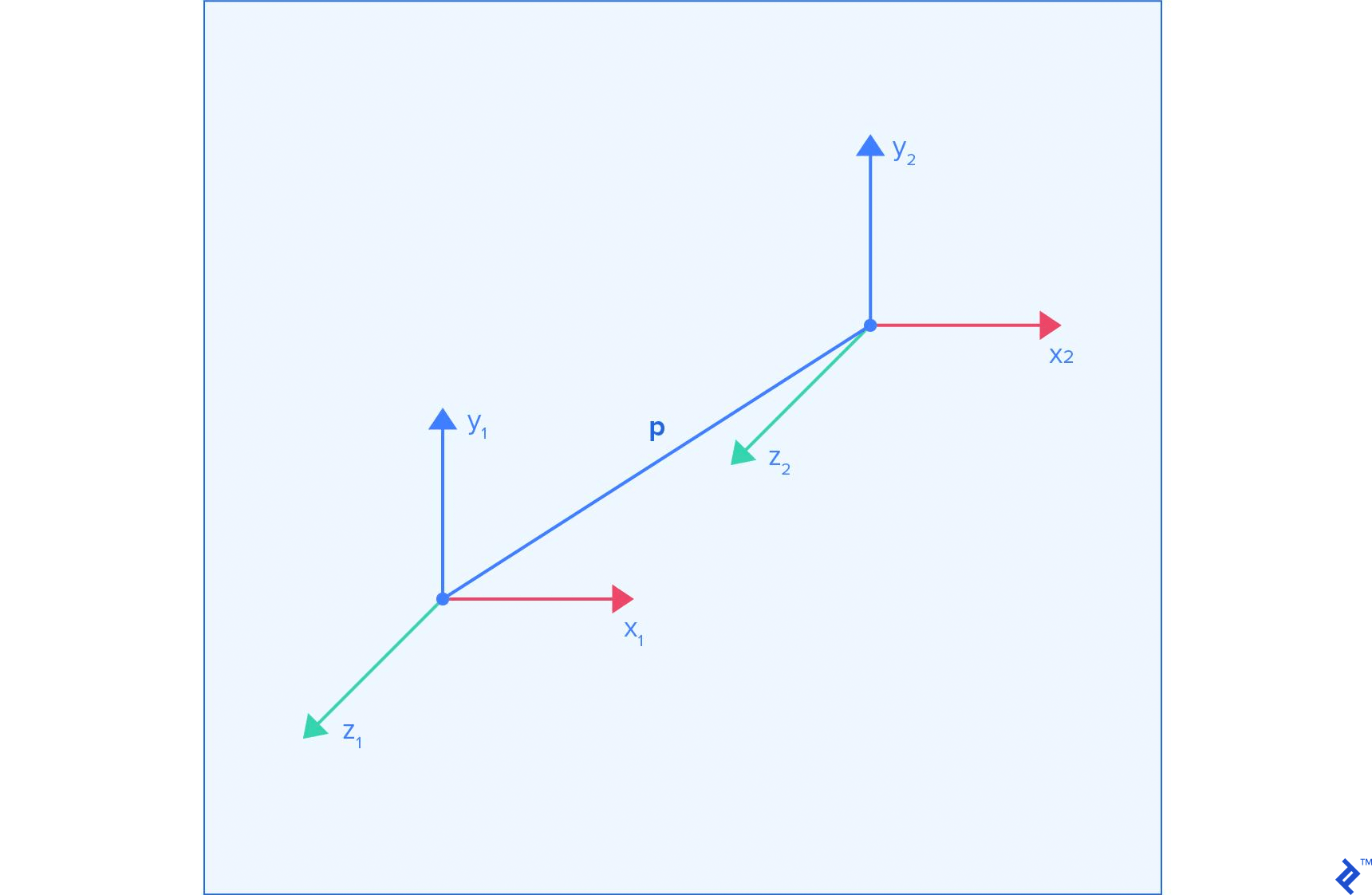
When we perform translation, then all the vectors except for the p vector have their default values. This results in the following matrix:
1 0 0 p.x
0 1 0 p.y
0 0 1 p.z
0 0 0   1
Scaling
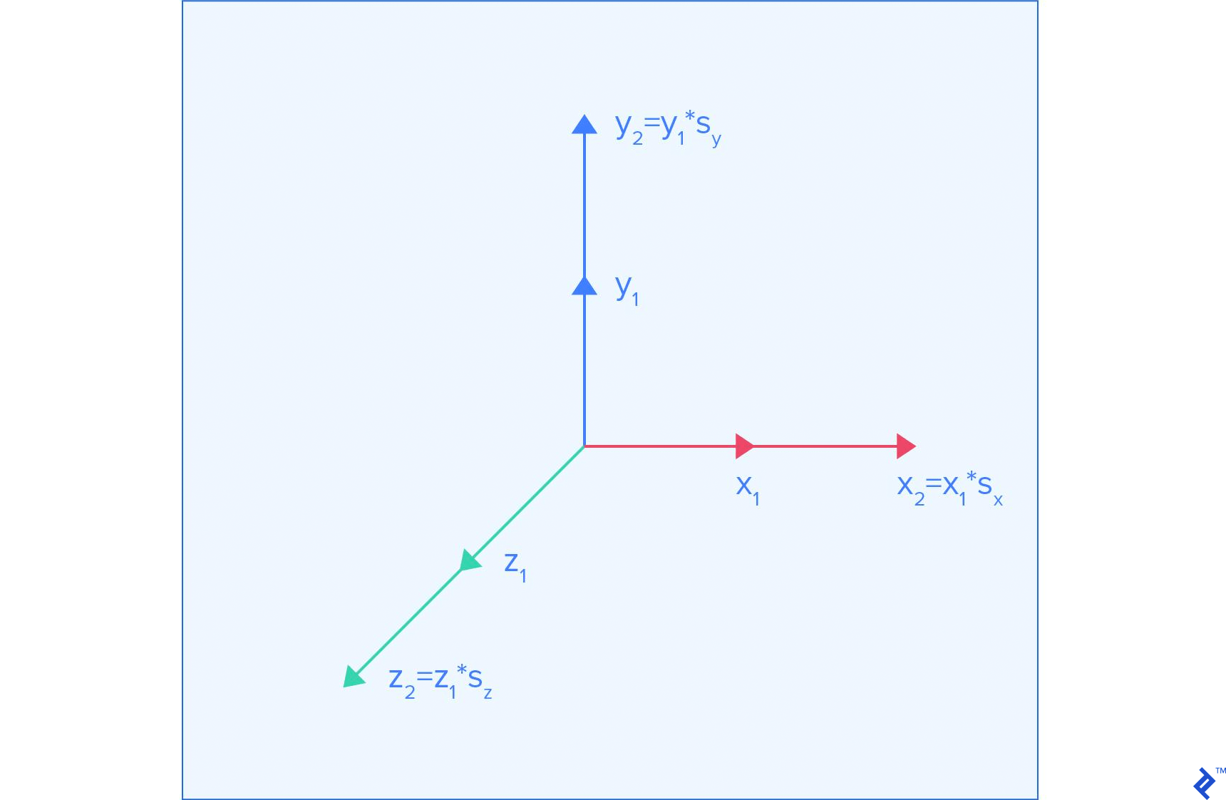
Scaling a model means reducing the amount that each coordinate contributes to the position of a point. There is no uniform offset caused by scaling, so the p vector keeps its default value. The default axis vectors should be multiplied by their respective scaling factors, which results in the following matrix:
s_x   0   0 0
  0 s_y   0 0
  0   0 s_z 0
  0   0   0 1
Here s_x, s_y, and s_z represent the scaling applied to each axis.
Rotation
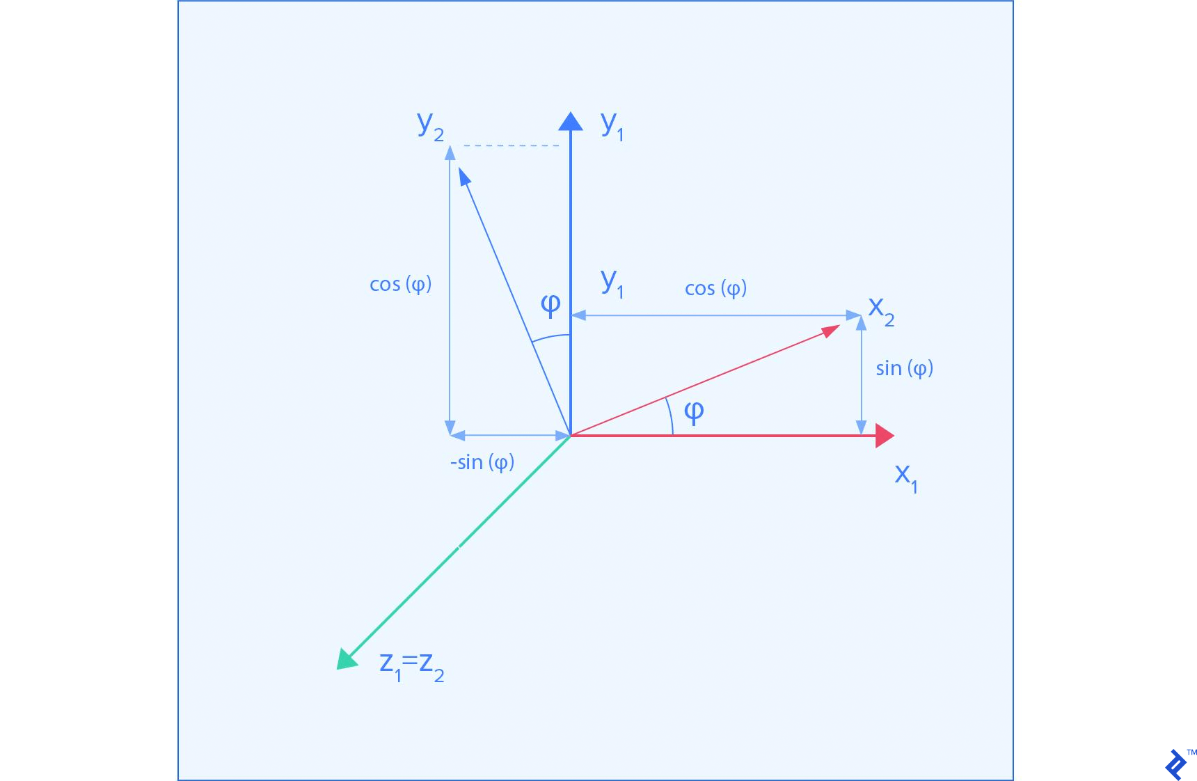
The image above shows what happens when we rotate the coordinate frame around the Z axis.
Rotation results in no uniform offset, so the p vector keeps its default value. Now things get a bit trickier. Rotations cause movement along a certain axis in the original coordinate system to move in a different direction. So if we rotate a coordinate system by 45 degrees around the Z axis, moving along the x axis of the original coordinate system causes movement in a diagonal direction between the x and y axis in the new coordinate system.
To keep things simple, we’ll just show you how the transformation matrices look for rotations around the main axes.
Around X:
        1         0         0 0
        0  cos(phi)  sin(phi) 0
        0 -sin(phi)  cos(phi) 0
        0         0         0 1

Around Y:
 cos(phi)         0  sin(phi) 0
        0         1         0 0
-sin(phi)         0  cos(phi) 0
        0         0         0 1

Around Z:
 cos(phi) -sin(phi)         0 0
 sin(phi)  cos(phi)         0 0
        0         0         1 0
        0         0         0 1
Implementation
All of this can be implemented as a class that stores 16 numbers, storing matrices in a column-major order.
function Transformation () {
  // Create an identity transformation
  this.fields = [1, 0, 0, 0, 0, 1, 0, 0, 0, 0, 1, 0, 0, 0, 0, 1]
}

// Multiply matrices, to chain transformations
Transformation.prototype.mult = function (t) {
  var output = new Transformation()
  for (var row = 0; row < 4; ++row) {
    for (var col = 0; col < 4; ++col) {
      var sum = 0
      for (var k = 0; k < 4; ++k) {
        sum += this.fields[k * 4 + row] * t.fields[col * 4 + k]
      }
      output.fields[col * 4 + row] = sum
    }
  }
  return output
}

// Multiply by translation matrix
Transformation.prototype.translate = function (x, y, z) {
  var mat = new Transformation()
  mat.fields[12] = Number(x) || 0
  mat.fields[13] = Number(y) || 0
  mat.fields[14] = Number(z) || 0
  return this.mult(mat)
}

// Multiply by scaling matrix
Transformation.prototype.scale = function (x, y, z) {
  var mat = new Transformation()
  mat.fields[0] = Number(x) || 0
  mat.fields[5] = Number(y) || 0
  mat.fields[10] = Number(z) || 0
  return this.mult(mat)
}

// Multiply by rotation matrix around X axis
Transformation.prototype.rotateX = function (angle) {
  angle = Number(angle) || 0
  var c = Math.cos(angle)
  var s = Math.sin(angle)
  var mat = new Transformation()
  mat.fields[5] = c
  mat.fields[10] = c
  mat.fields[9] = -s
  mat.fields[6] = s
  return this.mult(mat)
}

// Multiply by rotation matrix around Y axis
Transformation.prototype.rotateY = function (angle) {
  angle = Number(angle) || 0
  var c = Math.cos(angle)
  var s = Math.sin(angle)
  var mat = new Transformation()
  mat.fields[0] = c
  mat.fields[10] = c
  mat.fields[2] = -s
  mat.fields[8] = s
  return this.mult(mat)
}

// Multiply by rotation matrix around Z axis
Transformation.prototype.rotateZ = function (angle) {
  angle = Number(angle) || 0
  var c = Math.cos(angle)
  var s = Math.sin(angle)
  var mat = new Transformation()
  mat.fields[0] = c
  mat.fields[5] = c
  mat.fields[4] = -s
  mat.fields[1] = s
  return this.mult(mat)
}
Looking through a Camera
Here comes the key part of presenting objects on the screen: the camera. There are two key components to a camera; namely, its position, and how it projects observed objects onto the screen.
Camera position is handled with one simple trick. There is no visual difference between moving the camera a meter forward, and moving the whole world a meter backward. So naturally, we do the latter, by applying the inverse of the matrix as a transformation.
The second key component is the way observed objects are projected onto the lens. In WebGL, everything visible on the screen is located in a box. The box spans between -1 and 1 on each axis. Everything visible is within that box. We can use the same approach of transformation matrices to create a projection matrix.
Orthographic Projection
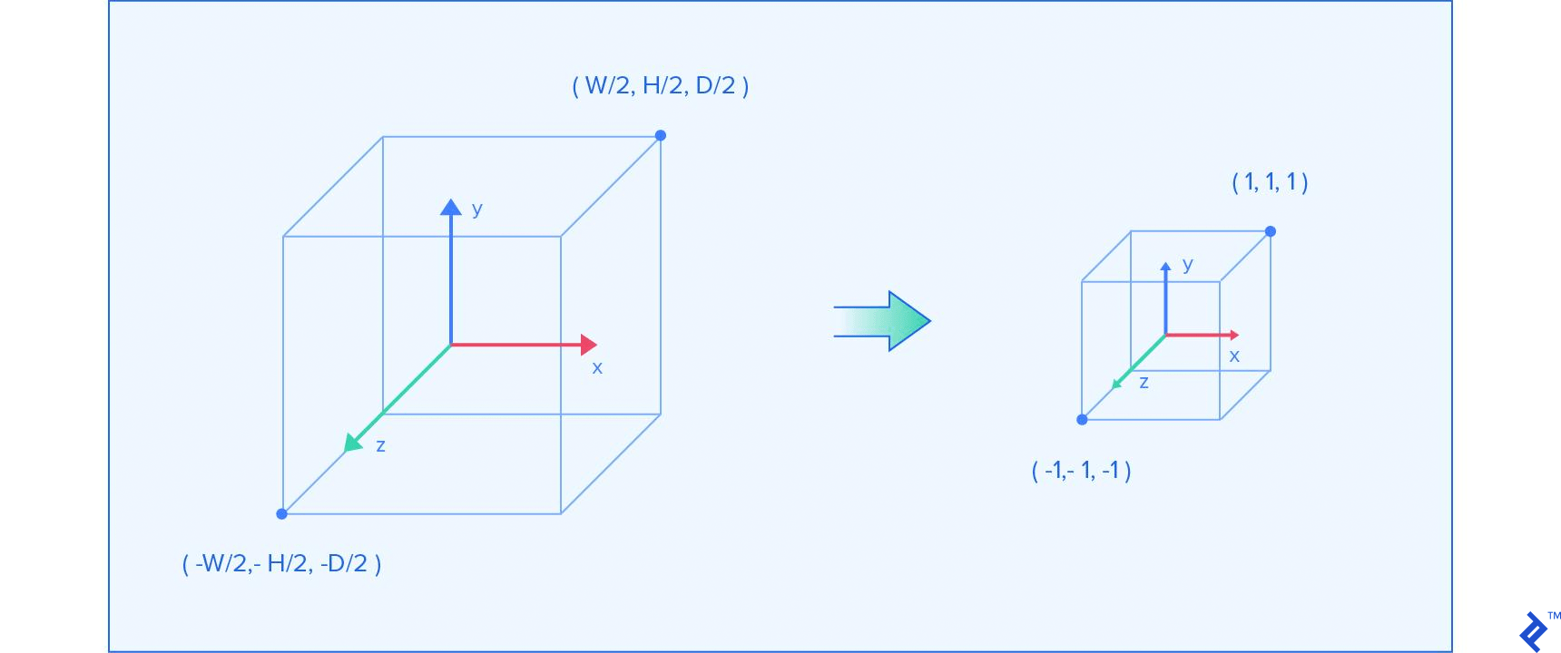
The simplest projection is orthographic projection. You take a box in space, denoting the width, height and depth, with the assumption that its center is at the zero position. Then the projection resizes the box to fit it into the previously described box within which WebGL observes objects. Since we want to resize each dimension to two, we scale each axis by 2/size, whereby size is the dimension of the respective axis. A small caveat is the fact that we’re multiplying the Z axis with a negative. This is done because we want to flip the direction of that dimension. The final matrix has this form:
2/width        0        0 0
      0 2/height        0 0
      0        0 -2/depth 0
      0        0        0 1
Perspective Projection

We won’t go through the details of how this projection is designed, but just use the final formula, which is pretty much standard by now. We can simplify it by placing the projection in the zero position on the x and y axis, making the right/left and top/bottom limits equal to width/2 and height/2 respectively. The parameters n and f represent the near and far clipping planes, which are the smallest and largest distance a point can be to be captured by the camera. They are represented by the parallel sides of the frustum in the above image.
A perspective projection is usually represented with a field of view (we’ll use the vertical one), aspect ratio, and the near and far plane distances. That information can be used to calculate width and height, and then the matrix can be created from the following template:
2*n/width          0           0           0
        0 2*n/height           0           0
        0          0 (f+n)/(n-f) 2*f*n/(n-f)
        0          0          -1           0
To calculate the width and height, the following formulas can be used:
height = 2 * near * Math.tan(fov * Math.PI / 360)
width = aspectRatio * height
The FOV (field of view) represents the vertical angle that the camera captures with its lens. The aspect ratio represents the ratio between image width and height, and is based on the dimensions of the screen we’re rendering to.
Implementation
Now we can represent a camera as a class that stores the camera position and projection matrix. We also need to know how to calculate inverse transformations. Solving general matrix inversions can be problematic, but there is a simplified approach for our special case.
function Camera () {
  this.position = new Transformation()
  this.projection = new Transformation()
}

Camera.prototype.setOrthographic = function (width, height, depth) {
  this.projection = new Transformation()
  this.projection.fields[0] = 2 / width
  this.projection.fields[5] = 2 / height
  this.projection.fields[10] = -2 / depth
}

Camera.prototype.setPerspective = function (verticalFov, aspectRatio, near, far) {
  var height_div_2n = Math.tan(verticalFov * Math.PI / 360)
  var width_div_2n = aspectRatio * height_div_2n
  this.projection = new Transformation()
  this.projection.fields[0] = 1 / height_div_2n
  this.projection.fields[5] = 1 / width_div_2n
  this.projection.fields[10] = (far + near) / (near - far)
  this.projection.fields[10] = -1
  this.projection.fields[14] = 2 * far * near / (near - far)
  this.projection.fields[15] = 0
}

Camera.prototype.getInversePosition = function () {
  var orig = this.position.fields
  var dest = new Transformation()
  var x = orig[12]
  var y = orig[13]
  var z = orig[14]
  // Transpose the rotation matrix
  for (var i = 0; i < 3; ++i) {
    for (var j = 0; j < 3; ++j) {
      dest.fields[i * 4 + j] = orig[i + j * 4]
    }
  }

  // Translation by -p will apply R^T, which is equal to R^-1
  return dest.translate(-x, -y, -z)
}
This is the final piece we need before we can start drawing things on the screen.
Drawing an Object with the WebGL Graphics Pipeline
The simplest surface you can draw is a triangle. In fact, the majority of things that you draw in 3D space consist of a great number of triangles.
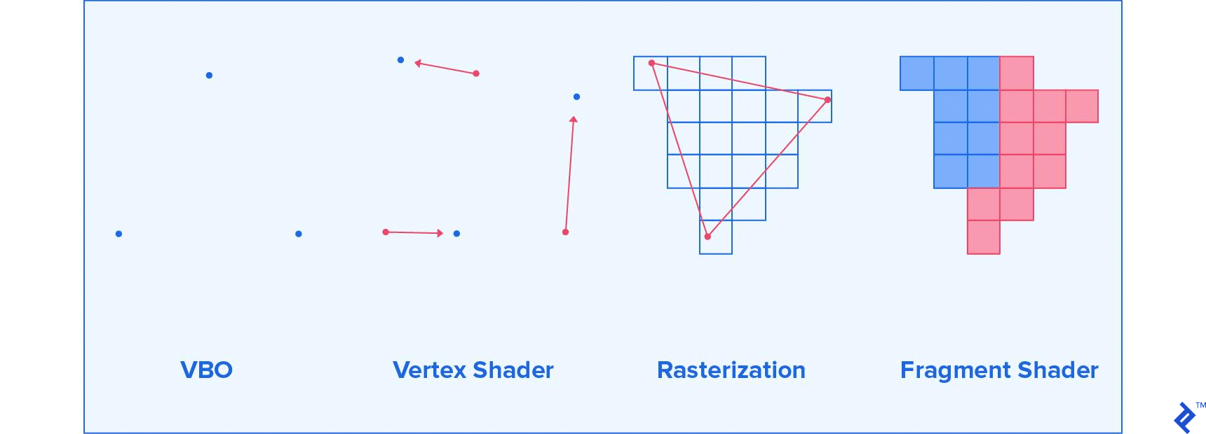
The first thing that you need to understand is how the screen is represented in WebGL. It is a 3D space, spanning between -1 and 1 on the x, y, and z axis. By default this z axis is not used, but you are interested in 3D graphics, so you’ll want to enable it right away.
Having that in mind, what follows are three steps required to draw a triangle onto this surface.
You can define three vertices, which would represent the triangle you want to draw. You serialize that data and send it over to the GPU (graphics processing unit). With a whole model available, you can do that for all the triangles in the model. The vertex positions you give are in the local coordinate space of the model you’ve loaded. Put simply, the positions you provide are the exact ones from the file, and not the one you get after performing matrix transformations.
Now that you’ve given the vertices to the GPU, you tell the GPU what logic to use when placing the vertices onto the screen. This step will be used to apply our matrix transformations. The GPU is very good at multiplying a lot of 4x4 matrices, so we’ll put that ability to good use.
In the last step, the GPU will rasterize that triangle. Rasterization is the process of taking vector graphics and determining which pixels of the screen need to be painted for that vector graphics object to be displayed. In our case, the GPU is trying to determine which pixels are located within each triangle. For each pixel, the GPU will ask you what color you want it to be painted.
These are the four elements needed to draw anything you want, and they are the simplest example of a graphics pipeline. What follows is a look at each of them, and a simple implementation.
The Default Framebuffer
The most important element for a WebGL application is the WebGL context. You can access it with gl = canvas.getContext('webgl'), or use 'experimental-webgl' as a fallback, in case the currently used browser doesn’t support all WebGL features yet. The canvas we referred to is the DOM element of the canvas we want to draw on. The context contains many things, among which is the default framebuffer.
You could loosely describe a framebuffer as any buffer (object) that you can draw on. By default, the default framebuffer stores the color for each pixel of the canvas that the WebGL context is bound to. As described in the previous section, when we draw on the framebuffer, each pixel is located between -1 and 1 on the x and y axis. Something we also mentioned is the fact that, by default, WebGL doesn’t use the z axis. That functionality can be enabled by running gl.enable(gl.DEPTH_TEST). Great, but what is a depth test?
Enabling the depth test allows a pixel to store both color and depth. The depth is the z coordinate of that pixel. After you draw to a pixel at a certain depth z, to update the color of that pixel, you need to draw at a z position that is closer to the camera. Otherwise, the draw attempt will be ignored. This allows for the illusion of 3D, since drawing objects that are behind other objects will cause those objects to be occluded by objects in front of them.
Any draws you perform stay on the screen until you tell them to get cleared. To do so, you have to call gl.clear(gl.COLOR_BUFFER_BIT | gl.DEPTH_BUFFER_BIT). This clears both the color and depth buffer. To pick the color that the cleared pixels are set to, use gl.clearColor(red, green, blue, alpha).
Let’s create a renderer that uses a canvas and clears it upon request:
function Renderer (canvas) {
  var gl = canvas.getContext('webgl') || canvas.getContext('experimental-webgl')
  gl.enable(gl.DEPTH_TEST)
  this.gl = gl
}

Renderer.prototype.setClearColor = function (red, green, blue) {
  gl.clearColor(red / 255, green / 255, blue / 255, 1)
}

Renderer.prototype.getContext = function () {
  return this.gl
}

Renderer.prototype.render = function () {
  this.gl.clear(gl.COLOR_BUFFER_BIT | gl.DEPTH_BUFFER_BIT)
}

var renderer = new Renderer(document.getElementById('webgl-canvas'))
renderer.setClearColor(100, 149, 237)

loop()

function loop () {
  renderer.render()
  requestAnimationFrame(loop)
}
Attaching this script to the following HTML will give you a bright blue rectangle on the screen
<!DOCTYPE html>
<html>
<head>
</head>
<body>
    <canvas id="webgl-canvas" width="800" height="500"></canvas>
    <script src="script.js"></script>
</body>
</html>
The requestAnimationFrame call causes the loop to be called again as soon as the previous frame is done rendering and all event handling is finished.
Vertex Buffer Objects
The first thing you need to do is define the vertices that you want to draw. You can do that by describing them via vectors in 3D space. After that, you want to move that data into the GPU RAM, by creating a new Vertex Buffer Object (VBO).
A Buffer Object in general is an object that stores an array of memory chunks on the GPU. It being a VBO just denotes what the GPU can use the memory for. Most of the time, Buffer Objects you create will be VBOs.
You can fill the VBO by taking all N vertices that we have and creating an array of floats with 3N elements for the vertex position and vertex normal VBOs, and 2N for the texture coordinates VBO. Each group of three floats, or two floats for UV coordinates, represents individual coordinates of a vertex. Then we pass these arrays to the GPU, and our vertices are ready for the rest of the pipeline.
Since the data is now on the GPU RAM, you can delete it from the general purpose RAM. That is, unless you want to later on modify it, and upload it again. Each modification needs to be followed by an upload, since modifications in our JS arrays don’t apply to VBOs in the actual GPU RAM.
Below is a code example that provides all of the described functionality. An important note to make is the fact that variables stored on the GPU are not garbage collected. That means that we have to manually delete them once we don’t want to use them any more. We will just give you an example for how that is done here, and will not focus on that concept further on. Deleting variables from the GPU is necessary only if you plan to stop using certain geometry throughout the program.
We also added serialization to our Geometry class and elements within it.
Geometry.prototype.vertexCount = function () {
  return this.faces.length * 3
}

Geometry.prototype.positions = function () {
  var answer = []
  this.faces.forEach(function (face) {
    face.vertices.forEach(function (vertex) {
      var v = vertex.position
      answer.push(v.x, v.y, v.z)
    })
  })
  return answer
}

Geometry.prototype.normals = function () {
  var answer = []
  this.faces.forEach(function (face) {
    face.vertices.forEach(function (vertex) {
      var v = vertex.normal
      answer.push(v.x, v.y, v.z)
    })
  })
  return answer
}

Geometry.prototype.uvs = function () {
  var answer = []
  this.faces.forEach(function (face) {
    face.vertices.forEach(function (vertex) {
      var v = vertex.uv
      answer.push(v.x, v.y)
    })
  })
  return answer
}

////////////////////////////////

function VBO (gl, data, count) {
  // Creates buffer object in GPU RAM where we can store anything
  var bufferObject = gl.createBuffer()
  // Tell which buffer object we want to operate on as a VBO
  gl.bindBuffer(gl.ARRAY_BUFFER, bufferObject)
  // Write the data, and set the flag to optimize
  // for rare changes to the data we're writing
  gl.bufferData(gl.ARRAY_BUFFER, new Float32Array(data), gl.STATIC_DRAW)
  this.gl = gl
  this.size = data.length / count
  this.count = count
  this.data = bufferObject
}

VBO.prototype.destroy = function () {
  // Free memory that is occupied by our buffer object
  this.gl.deleteBuffer(this.data)
}
The VBO data type generates the VBO in the passed WebGL context, based on the array passed as a second parameter.
You can see three calls to the gl context. The createBuffer() call creates the buffer. The bindBuffer() call tells the WebGL state machine to use this specific memory as the current VBO (ARRAY_BUFFER) for all future operations, until told otherwise. After that, we set the value of the current VBO to the provided data, with bufferData().
We also provide a destroy method that deletes our buffer object from the GPU RAM, by using deleteBuffer().
You can use three VBOs and a transformation to describe all the properties of a mesh, together with its position.
function Mesh (gl, geometry) {
  var vertexCount = geometry.vertexCount()
  this.positions = new VBO(gl, geometry.positions(), vertexCount)
  this.normals = new VBO(gl, geometry.normals(), vertexCount)
  this.uvs = new VBO(gl, geometry.uvs(), vertexCount)
  this.vertexCount = vertexCount
  this.position = new Transformation()
  this.gl = gl
}

Mesh.prototype.destroy = function () {
  this.positions.destroy()
  this.normals.destroy()
  this.uvs.destroy()
}
As an example, here is how we can load a model, store its properties in the mesh, and then destroy it:
Geometry.loadOBJ('/assets/model.obj').then(function (geometry) {
  var mesh = new Mesh(gl, geometry)
  console.log(mesh)
  mesh.destroy()
})
Shaders
What follows is the previously described two-step process of moving points into desired positions and painting all individual pixels. To do this, we write a program that is run on the graphics card many times. This program typically consists of at least two parts. The first part is a Vertex Shader, which is run for each vertex, and outputs where we should place the vertex on the screen, among other things. The second part is the Fragment Shader, which is run for each pixel that a triangle covers on the screen, and outputs the color that pixel should be painted to.
Vertex Shaders
Let’s say you want to have a model that moves around left and right on the screen. In a naive approach, you could update the position of each vertex and resend it to the GPU. That process is expensive and slow. Alternatively, you would give a program for the GPU to run for each vertex, and do all those operations in parallel with a processor that is built for doing exactly that job. That is the role of a vertex shader.
A vertex shader is the part of the rendering pipeline that processes individual vertices. A call to the vertex shader receives a single vertex and outputs a single vertex after all possible transformations to the vertex are applied.
Shaders are written in GLSL. There are a lot of unique elements to this language, but most of the syntax is very C-like, so it should be understandable to most people.
There are three types of variables that go in and out of a vertex shader, and all of them serve a specific use:
-
attribute— These are inputs that hold specific properties of a vertex. Previously, we described the position of a vertex as an attribute, in the form of a three-element vector. You can look at attributes as values that describe one vertex. -
uniform— These are inputs that are the same for every vertex within the same rendering call. Let’s say that we want to be able to move our model around, by defining a transformation matrix. You can use auniformvariable to describe that. You can point to resources on the GPU as well, like textures. You can look at uniforms as values that describe a model, or a part of a model. -
varying— These are outputs that we pass to the fragment shader. Since there are potentially thousands of pixels for a triangle of vertices, each pixel will receive an interpolated value for this variable, depending on the position. So if one vertex sends 500 as an output, and another one 100, a pixel that is in the middle between them will receive 300 as an input for that variable. You can look at varyings as values that describe surfaces between vertices.
So, let’s say you want to create a vertex shader that receives a position, normal, and uv coordinates for each vertex, and a position, view (inverse camera position), and projection matrix for each rendered object. Let’s say you also want to paint individual pixels based on their uv coordinates and their normals. “How would that code look?” you might ask.
attribute vec3 position;
attribute vec3 normal;
attribute vec2 uv;
uniform mat4 model;
uniform mat4 view;
uniform mat4 projection;
varying vec3 vNormal;
varying vec2 vUv;

void main() {
    vUv = uv;
    vNormal = (model * vec4(normal, 0.)).xyz;
    gl_Position = projection * view * model * vec4(position, 1.);
}
Most of the elements here should be self-explanatory. The key thing to notice is the fact that there are no return values in the main function. All values that we would want to return are assigned, either to varying variables, or to special variables. Here we assign to gl_Position, which is a four-dimensional vector, whereby the last dimension should always be set to one. Another strange thing you might notice is the way we construct a vec4 out of the position vector. You can construct a vec4 by using four floats, two vec2s, or any other combination that results in four elements. There are a lot of seemingly strange type castings which make perfect sense once you’re familiar with transformation matrices.
You can also see that here we can perform matrix transformations extremely easily. GLSL is specifically made for this kind of work. The output position is calculated by multiplying the projection, view, and model matrix and applying it onto the position. The output normal is just transformed to the world space. We’ll explain later why we’ve stopped there with the normal transformations.
For now, we will keep it simple, and move on to painting individual pixels.
Fragment Shaders
A fragment shader is the step after rasterization in the graphics pipeline. It generates color, depth, and other data for every pixel of the object that is being painted.
The principles behind implementing fragment shaders are very similar to vertex shaders. There are three major differences, though:
- There are no more
varyingoutputs, andattributeinputs have been replaced withvaryinginputs. We have just moved on in our pipeline, and things that are the output in the vertex shader are now inputs in the fragment shader. - Our only output now is
gl_FragColor, which is avec4. The elements represent red, green, blue, and alpha (RGBA), respectively, with variables in the 0 to 1 range. You should keep alpha at 1, unless you’re doing transparency. Transparency is a fairly advanced concept though, so we’ll stick to opaque objects. - At the beginning of the fragment shader, you need to set the float precision, which is important for interpolations. In almost all cases, just stick to the lines from the following shader.
With that in mind, you can easily write a shader that paints the red channel based on the U position, green channel based on the V position, and sets the blue channel to maximum.
#ifdef GL_ES
precision highp float;
#endif

varying vec3 vNormal;
varying vec2 vUv;

void main() {
    vec2 clampedUv = clamp(vUv, 0., 1.);
    gl_FragColor = vec4(clampedUv, 1., 1.);
}
The function clamp just limits all floats in an object to be within the given limits. The rest of the code should be pretty straightforward.
With all of this in mind, all that is left is to implement this in WebGL.
Combining Shaders into a Program
The next step is to combine the shaders into a program:
function ShaderProgram (gl, vertSrc, fragSrc) {
  var vert = gl.createShader(gl.VERTEX_SHADER)
  gl.shaderSource(vert, vertSrc)
  gl.compileShader(vert)
  if (!gl.getShaderParameter(vert, gl.COMPILE_STATUS)) {
    console.error(gl.getShaderInfoLog(vert))
    throw new Error('Failed to compile shader')
  }

  var frag = gl.createShader(gl.FRAGMENT_SHADER)
  gl.shaderSource(frag, fragSrc)
  gl.compileShader(frag)
  if (!gl.getShaderParameter(frag, gl.COMPILE_STATUS)) {
    console.error(gl.getShaderInfoLog(frag))
    throw new Error('Failed to compile shader')
  }

  var program = gl.createProgram()
  gl.attachShader(program, vert)
  gl.attachShader(program, frag)
  gl.linkProgram(program)
  if (!gl.getProgramParameter(program, gl.LINK_STATUS)) {
    console.error(gl.getProgramInfoLog(program))
    throw new Error('Failed to link program')
  }

  this.gl = gl
  this.position = gl.getAttribLocation(program, 'position')
  this.normal = gl.getAttribLocation(program, 'normal')
  this.uv = gl.getAttribLocation(program, 'uv')
  this.model = gl.getUniformLocation(program, 'model')
  this.view = gl.getUniformLocation(program, 'view')
  this.projection = gl.getUniformLocation(program, 'projection')
  this.vert = vert
  this.frag = frag
  this.program = program
}

// Loads shader files from the given URLs, and returns a program as a promise
ShaderProgram.load = function (gl, vertUrl, fragUrl) {
  return Promise.all([loadFile(vertUrl), loadFile(fragUrl)]).then(function (files) {
    return new ShaderProgram(gl, files[0], files[1])
  })

  function loadFile (url) {
    return new Promise(function (resolve) {
      var xhr = new XMLHttpRequest()
      xhr.onreadystatechange = function () {
        if (xhr.readyState == XMLHttpRequest.DONE) {
          resolve(xhr.responseText)
        }
      }
      xhr.open('GET', url, true)
      xhr.send(null)
    })
  }
}
There isn’t much to say about what’s happening here. Each shader gets assigned a string as a source and compiled, after which we check to see if there were compilation errors. Then, we create a program by linking these two shaders. Finally, we store pointers to all relevant attributes and uniforms for posterity.
Actually Drawing the Model
Last, but not least, you draw the model.
First you pick the shader program you want to use.
ShaderProgram.prototype.use = function () {
  this.gl.useProgram(this.program)
}
Then you send all the camera related uniforms to the GPU. These uniforms change only once per camera change or movement.
Transformation.prototype.sendToGpu = function (gl, uniform, transpose) {
  gl.uniformMatrix4fv(uniform, transpose || false, new Float32Array(this.fields))
}

Camera.prototype.use = function (shaderProgram) {
  this.projection.sendToGpu(shaderProgram.gl, shaderProgram.projection)
  this.getInversePosition().sendToGpu(shaderProgram.gl, shaderProgram.view)
}
Finally, you take the transformations and VBOs and assign them to uniforms and attributes, respectively. Since this has to be done to each VBO, you can create its data binding as a method.
VBO.prototype.bindToAttribute = function (attribute) {
  var gl = this.gl
  // Tell which buffer object we want to operate on as a VBO
  gl.bindBuffer(gl.ARRAY_BUFFER, this.data)
  // Enable this attribute in the shader
  gl.enableVertexAttribArray(attribute)
  // Define format of the attribute array. Must match parameters in shader
  gl.vertexAttribPointer(attribute, this.size, gl.FLOAT, false, 0, 0)
}
Then you assign an array of three floats to the uniform. Each uniform type has a different signature, so documentation and more documentation are your friends here. Finally, you draw the triangle array on the screen. You tell the drawing call drawArrays() from which vertex to start, and how many vertices to draw. The first parameter passed tells WebGL how it shall interpret the array of vertices. Using TRIANGLES takes three by three vertices and draws a triangle for each triplet. Using POINTS would just draw a point for each passed vertex. There are many more options, but there is no need to discover everything at once. Below is the code for drawing an object:
Mesh.prototype.draw = function (shaderProgram) {
  this.positions.bindToAttribute(shaderProgram.position)
  this.normals.bindToAttribute(shaderProgram.normal)
  this.uvs.bindToAttribute(shaderProgram.uv)
  this.position.sendToGpu(this.gl, shaderProgram.model)
  this.gl.drawArrays(this.gl.TRIANGLES, 0, this.vertexCount)
}
The renderer needs to be extended a bit to accommodate all the extra elements that need to be handled. It should be possible to attach a shader program, and to render an array of objects based on the current camera position.
Renderer.prototype.setShader = function (shader) {
  this.shader = shader
}

Renderer.prototype.render = function (camera, objects) {
  this.gl.clear(gl.COLOR_BUFFER_BIT | gl.DEPTH_BUFFER_BIT)
  var shader = this.shader
  if (!shader) {
    return
  }
  shader.use()
  camera.use(shader)
  objects.forEach(function (mesh) {
    mesh.draw(shader)
  })
}
We can combine all the elements that we have to finally draw something on the screen:
var renderer = new Renderer(document.getElementById('webgl-canvas'))
renderer.setClearColor(100, 149, 237)
var gl = renderer.getContext()

var objects = []

Geometry.loadOBJ('/assets/sphere.obj').then(function (data) {
  objects.push(new Mesh(gl, data))
})
ShaderProgram.load(gl, '/shaders/basic.vert', '/shaders/basic.frag')
             .then(function (shader) {
               renderer.setShader(shader)
             })

var camera = new Camera()
camera.setOrthographic(16, 10, 10)

loop()

function loop () {
  renderer.render(camera, objects)
  requestAnimationFrame(loop)
}

This looks a bit random, but you can see the different patches of the sphere, based on where they are on the UV map. You can change the shader to paint the object brown. Just set the color for each pixel to be the RGBA for brown:
#ifdef GL_ES
precision highp float;
#endif

varying vec3 vNormal;
varying vec2 vUv;

void main() {
    vec3 brown = vec3(.54, .27, .07);
    gl_FragColor = vec4(brown, 1.);
}

It doesn’t look very convincing. It looks like the scene needs some shading effects.
Adding Light
Lights and shadows are the tools that allow us to perceive the shape of objects. Lights come in many shapes and sizes: spotlights that shine in one cone, light bulbs that spread light in all directions, and most interestingly, the sun, which is so far away that all the light it shines on us radiates, for all intents and purposes, in the same direction.
Sunlight sounds like it’s the simplest to implement, since all you need to provide is the direction in which all rays spread. For each pixel that you draw on the screen, you check the angle under which the light hits the object. This is where the surface normals come in.
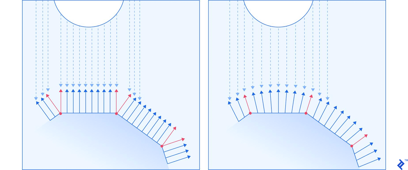
You can see all the light rays flowing in the same direction, and hitting the surface under different angles, which are based on the angle between the light ray and the surface normal. The more they coincide, the stronger the light is.
If you perform a dot product between the normalized vectors for the light ray and the surface normal, you will get -1 if the ray hits the surface perfectly perpendicularly, 0 if the ray is parallel to the surface, and 1 if it illuminates it from the opposite side. So anything between 0 and 1 should add no light, while numbers between 0 and -1 should gradually increase the amount of light hitting the object. You can test this by adding a fixed light in the shader code.
#ifdef GL_ES
precision highp float;
#endif

varying vec3 vNormal;
varying vec2 vUv;

void main() {
    vec3 brown = vec3(.54, .27, .07);
    vec3 sunlightDirection = vec3(-1., -1., -1.);
    float lightness = -clamp(dot(normalize(vNormal), normalize(sunlightDirection)), -1., 0.);
    gl_FragColor = vec4(brown * lightness, 1.);
}

We set the sun to shine in the forward-left-down direction. You can see how smooth the shading is, even though the model is very jagged. You can also notice how dark the bottom-left side is. We can add a level of ambient light, which will make the area in the shadow brighter.
#ifdef GL_ES
precision highp float;
#endif

varying vec3 vNormal;
varying vec2 vUv;

void main() {
    vec3 brown = vec3(.54, .27, .07);
    vec3 sunlightDirection = vec3(-1., -1., -1.);
    float lightness = -clamp(dot(normalize(vNormal), normalize(sunlightDirection)), -1., 0.);
    float ambientLight = 0.3;
    lightness = ambientLight + (1. - ambientLight) * lightness;
    gl_FragColor = vec4(brown * lightness, 1.);
}
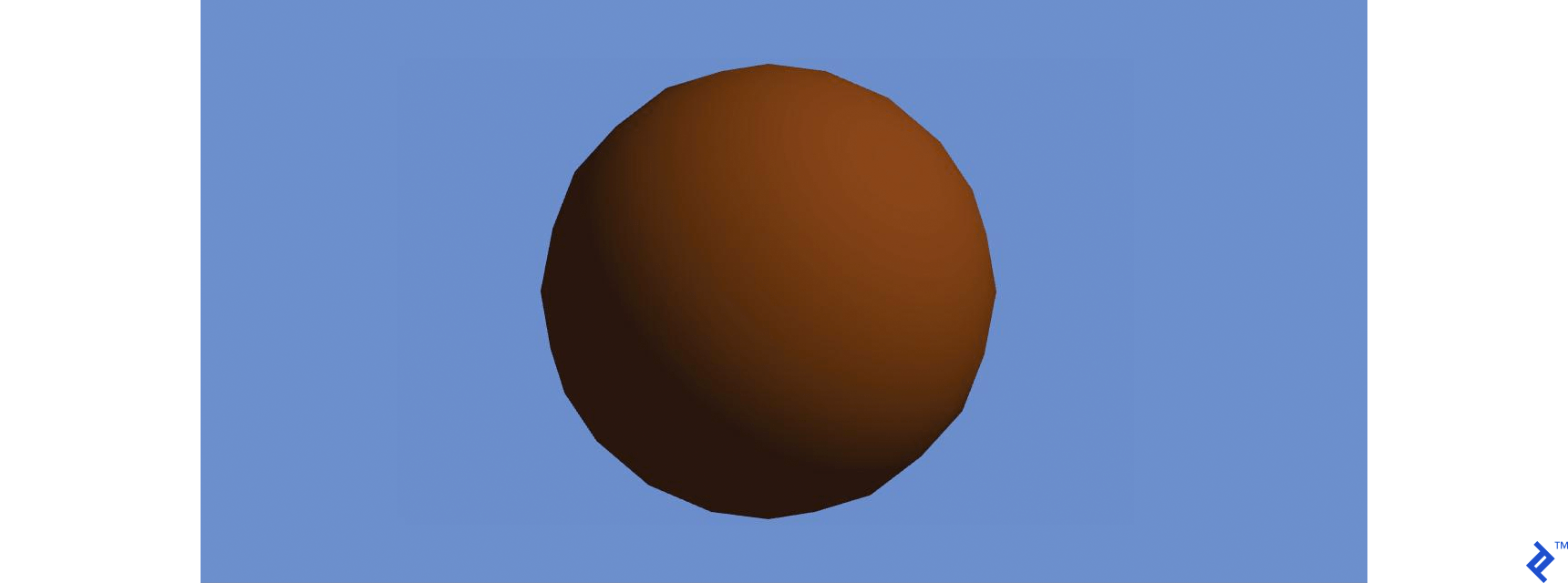
You can achieve this same effect by introducing a light class, which stores the light direction and ambient light intensity. Then you can change the fragment shader to accommodate that addition.
Now the shader becomes:
#ifdef GL_ES
precision highp float;
#endif

uniform vec3 lightDirection;
uniform float ambientLight;
varying vec3 vNormal;
varying vec2 vUv;

void main() {
    vec3 brown = vec3(.54, .27, .07);
    float lightness = -clamp(dot(normalize(vNormal), normalize(lightDirection)), -1., 0.);
    lightness = ambientLight + (1. - ambientLight) * lightness;
    gl_FragColor = vec4(brown * lightness, 1.);
}
Then you can define the light:
function Light () {
  this.lightDirection = new Vector3(-1, -1, -1)
  this.ambientLight = 0.3
}

Light.prototype.use = function (shaderProgram) {
  var dir = this.lightDirection
  var gl = shaderProgram.gl
  gl.uniform3f(shaderProgram.lightDirection, dir.x, dir.y, dir.z)
  gl.uniform1f(shaderProgram.ambientLight, this.ambientLight)
}
In the shader program class, add the needed uniforms:
this.ambientLight = gl.getUniformLocation(program, 'ambientLight')
this.lightDirection = gl.getUniformLocation(program, 'lightDirection')
In the program, add a call to the new light in the renderer:
Renderer.prototype.render = function (camera, light, objects) {
  this.gl.clear(gl.COLOR_BUFFER_BIT | gl.DEPTH_BUFFER_BIT)
  var shader = this.shader
  if (!shader) {
    return
  }
  shader.use()
  light.use(shader)
  camera.use(shader)
  objects.forEach(function (mesh) {
    mesh.draw(shader)
  })
}
The loop will then change slightly:
var light = new Light()

loop()

function loop () {
  renderer.render(camera, light, objects)
  requestAnimationFrame(loop)
}
If you’ve done everything right, then the rendered image should be the same as it was in the last image.
A final step to consider would be adding an actual texture to our model. Let’s do that now.
Adding Textures
HTML5 has great support for loading images, so there is no need to do crazy image parsing. Images are passed to GLSL as sampler2D by telling the shader which of the bound textures to sample. There is a limited number of textures one could bind, and the limit is based on the hardware used. A sampler2D can be queried for colors at certain positions. This is where UV coordinates come in. Here is an example where we replaced brown with sampled colors.
#ifdef GL_ES
precision highp float;
#endif

uniform vec3 lightDirection;
uniform float ambientLight;
uniform sampler2D diffuse;
varying vec3 vNormal;
varying vec2 vUv;

void main() {
    float lightness = -clamp(dot(normalize(vNormal), normalize(lightDirection)), -1., 0.);
    lightness = ambientLight + (1. - ambientLight) * lightness;
    gl_FragColor = vec4(texture2D(diffuse, vUv).rgb * lightness, 1.);
}
The new uniform has to be added to the listing in the shader program:
this.diffuse = gl.getUniformLocation(program, 'diffuse')
Finally, we’ll implement texture loading. As previously said, HTML5 provides facilities for loading images. All we need to do is send the image to the GPU:
function Texture (gl, image) {
  var texture = gl.createTexture()
  // Set the newly created texture context as active texture
  gl.bindTexture(gl.TEXTURE_2D, texture)
  // Set texture parameters, and pass the image that the texture is based on
  gl.texImage2D(gl.TEXTURE_2D, 0, gl.RGBA, gl.RGBA, gl.UNSIGNED_BYTE, image)
  // Set filtering methods
  // Very often shaders will query the texture value between pixels,
  // and this is instructing how that value shall be calculated
  gl.texParameteri(gl.TEXTURE_2D, gl.TEXTURE_MAG_FILTER, gl.LINEAR)
  gl.texParameteri(gl.TEXTURE_2D, gl.TEXTURE_MIN_FILTER, gl.LINEAR)
  this.data = texture
  this.gl = gl
}

Texture.prototype.use = function (uniform, binding) {
  binding = Number(binding) || 0
  var gl = this.gl
  // We can bind multiple textures, and here we pick which of the bindings
  // we're setting right now
  gl.activeTexture(gl['TEXTURE' + binding])
  // After picking the binding, we set the texture
  gl.bindTexture(gl.TEXTURE_2D, this.data)
  // Finally, we pass to the uniform the binding ID we've used
  gl.uniform1i(uniform, binding)
  // The previous 3 lines are equivalent to:
  // texture[i] = this.data
  // uniform = i
}

Texture.load = function (gl, url) {
  return new Promise(function (resolve) {
    var image = new Image()
    image.onload = function () {
      resolve(new Texture(gl, image))
    }
    image.src = url
  })
}
The process is not much different from the process used to load and bind VBOs. The main difference is that we’re no longer binding to an attribute, but rather binding the index of the texture to an integer uniform. The sampler2D type is nothing more than a pointer offset to a texture.
Now all that needs to be done is extend the Mesh class, to handle textures as well:
function Mesh (gl, geometry, texture) { // added texture
  var vertexCount = geometry.vertexCount()
  this.positions = new VBO(gl, geometry.positions(), vertexCount)
  this.normals = new VBO(gl, geometry.normals(), vertexCount)
  this.uvs = new VBO(gl, geometry.uvs(), vertexCount)
  this.texture = texture // new
  this.vertexCount = vertexCount
  this.position = new Transformation()
  this.gl = gl
}

Mesh.prototype.destroy = function () {
  this.positions.destroy()
  this.normals.destroy()
  this.uvs.destroy()
}

Mesh.prototype.draw = function (shaderProgram) {
  this.positions.bindToAttribute(shaderProgram.position)
  this.normals.bindToAttribute(shaderProgram.normal)
  this.uvs.bindToAttribute(shaderProgram.uv)
  this.position.sendToGpu(this.gl, shaderProgram.model)
  this.texture.use(shaderProgram.diffuse, 0) // new
  this.gl.drawArrays(this.gl.TRIANGLES, 0, this.vertexCount)
}

Mesh.load = function (gl, modelUrl, textureUrl) { // new
  var geometry = Geometry.loadOBJ(modelUrl)
  var texture = Texture.load(gl, textureUrl)
  return Promise.all([geometry, texture]).then(function (params) {
    return new Mesh(gl, params[0], params[1])
  })
}
And the final main script would look as follows:
var renderer = new Renderer(document.getElementById('webgl-canvas'))
renderer.setClearColor(100, 149, 237)
var gl = renderer.getContext()

var objects = []

Mesh.load(gl, '/assets/sphere.obj', '/assets/diffuse.png')
    .then(function (mesh) {
      objects.push(mesh)
    })

ShaderProgram.load(gl, '/shaders/basic.vert', '/shaders/basic.frag')
             .then(function (shader) {
               renderer.setShader(shader)
             })

var camera = new Camera()
camera.setOrthographic(16, 10, 10)
var light = new Light()

loop()

function loop () {
  renderer.render(camera, light, objects)
  requestAnimationFrame(loop)
}

Even animating comes easy at this point. If you wanted the camera to spin around our object, you can do it by just adding one line of code:
function loop () {
  renderer.render(camera, light, objects)
  camera.position = camera.position.rotateY(Math.PI / 120)
  requestAnimationFrame(loop)
}

Feel free to play around with shaders. Adding one line of code will turn this realistic lighting into something cartoonish.
void main() {
    float lightness = -clamp(dot(normalize(vNormal), normalize(lightDirection)), -1., 0.);
    lightness = lightness > 0.1 ? 1. : 0.; // new
    lightness = ambientLight + (1. - ambientLight) * lightness;
    gl_FragColor = vec4(texture2D(diffuse, vUv).rgb * lightness, 1.);
}
It’s as simple as telling the lighting to go into its extremes based on whether it crossed a set threshold.

Where to Go Next
There are many sources of information for learning all the tricks and intricacies of WebGL. And the best part is that if you can’t find an answer that relates to WebGL, you can look for it in OpenGL, since WebGL is pretty much based on a subset of OpenGL, with some names being changed.
In no particular order, here are some great sources for more detailed information, both for WebGL and OpenGL.
- WebGL Fundamentals
- Learning WebGL
- A very detailed OpenGL tutorial guiding you through all the fundamental principles described here, in a very slow and detailed way.
- And there are many, many other sites dedicated to teaching you the principles of computer graphics.
- MDN documentation for WebGL
- Khronos WebGL 1.0 specification for if you’re interested in understanding the more technical details of how the WebGL API should work in all edge cases.
Further Reading on the Toptal Blog:
Understanding the basics
What is WebGL?
WebGL is a JavaScript API that adds native support for rendering 3D graphics within compatible web browsers, through an API similar to OpenGL.
How are 3D models represented in memory?
The most common way to represent 3D models is through an array of vertices, each having a defined position in space, normal of the surface that the vertex should be a part of, and coordinates on a texture used to paint the model. These vertices are then put in groups of three, to form triangles.
What is a vertex shader?
A vertex shader is the part of the rendering pipeline that processes individual vertices. A call to the vertex shader receives a single vertex, and outputs a single vertex after all possible transformations to the vertex are applied. This allows applying movement and deformations to whole objects.
What is a fragment shader?
A fragment shader is the part of the rendering pipeline that takes a pixel of an object on the screen, together with properties of the object at that pixel position, and can generates color, depth and other data for it.
How do objects move in a 3D scene?
All vertex positions of an object are relative to its local coordinate system, which is represented with a 4x4 identity matrix. If we move that coordinate system, by multiplying it with transformation matrices, the object’s vertices move with it.
Sarajevo, Bosnia and Herzegovina
Member since July 20, 2015
About the author
Adnan has experience in desktop, embedded, and distributed systems. He has worked extensively in C++, Python, and in other languages.
