Embeddings in Machine Learning: Making Complex Data Simple
Working with non-numerical data can be challenging, even for seasoned data scientists. To make good use of such data, it needs to be transformed. But how?
In this article, Toptal Data Scientist Yaroslav Kopotilov will introduce you to embeddings and demonstrate how they can be used to visualize complex data and make it usable.
Yaroslav is a data scientist with experience in business analysis, predictive modeling, data visualization, data orchestration, and deployment.
Expertise
PREVIOUSLY AT

Working with non-numerical data can be tough, even for experienced data scientists. A typical machine learning model expects its features to be numbers, not words, emails, website pages, lists, graphs, or probability distributions. To be useful, data has to be transformed into a vector space first. But how?
One popular approach would be to treat a non-numerical feature as categorical. This could work well if the number of categories is small (for example, if data indicates a profession or a country). However, if we try to apply this method to emails, we will likely get as many categories as there are samples. No two emails are exactly the same, hence this approach would be of no use.
Another approach would be to define a distance between data samples, a function that tells us how close any two samples are. Or we could define a similarity measure, which would give us the same information except that the distance between two close samples is small while similarity is large. Computing distance (similarity) between all data samples would give us a distance (or similarity) matrix. This is numerical data we could use.
However, this data would have as many dimensions as there are samples, which is usually not great if we want to use it as a feature (see curse of dimensionality) or to visualize it (while one plot can handle even 6D, I have yet to see a 100D plot). Could we reduce the number of dimensions to a reasonable amount?
The answer is yes! That’s what we have embeddings for.
What Is an Embedding and Why Use It?
An embedding is a low-dimensional representation of high-dimensional data. Typically, an embedding won’t capture all information contained in the original data. A good embedding, however, will capture enough to solve the problem at hand.
There exist many embeddings tailored for a particular data structure. For example, you might have heard of word2vec for text data, or Fourier descriptors for shape image data. Instead, we will discuss how to apply embeddings to any data where we can define a distance or a similarity measure. As long as we can compute a distance matrix, the nature of data is completely irrelevant. It will work the same, be it emails, lists, trees, or web pages.
In this article, we will introduce you to different types of embedding and discuss how some popular embeddings work and how we could use embeddings to solve real-world problems involving complex data. We will also go through the pros and cons of this method, as well as some alternatives. Yes, some problems can be solved better by other means, but unfortunately, there is no silver bullet in machine learning.
Let’s get started.
How Embeddings Work
All embeddings attempt to reduce the dimensionality of data while preserving “essential” information in the data, but every embedding does it in its own way. Here, we will go through a few popular embeddings that can be applied to a distance or similarity matrix.
We won’t even attempt to cover all the embeddings out there. There are at least a dozen well-known embeddings that can do that and many more lesser-known embeddings and their variations. Each of them has its own approach, advantages, and disadvantages.
If you’d like to see what other embeddings are out there, you could start here:
Distance Matrix
Let’s briefly touch on distance matrices. Finding an appropriate distance for data requires a good understanding of the problem, some knowledge of math, and sometimes sheer luck. In the approach described in this article, that might be the most important factor contributing to the overall success or failure of your project.
You should also keep a few technical details in mind. Many embedding algorithms will assume that a distance (or dissimilarity) matrix $\textbf{D}$ has zeros on its diagonal and is symmetric. If it’s not symmetric, we can use $(\textbf{D} + \textbf{D}^T) / 2$ instead. Algorithms using the kernel trick will also assume that a distance is a metric, which means that the triangle inequality holds:
\[\forall a, b, c \;\; d(a,c) \leq d(a,b) + d(b,c)\]Also, if an algorithm requires a similarity matrix instead, we could apply any monotone-decreasing function to transform a distance matrix to a similarity matrix: for example, $\exp -x$.
Principal Component Analysis (PCA)
Principal Component Analysis, or PCA, is probably the most widely used embedding to date. The idea is simple: Find a linear transformation of features that maximizes the captured variance or (equivalently) minimizes the quadratic reconstruction error.
Specifically, let features be a sample matrix $\textbf{X} \in \mathbb{R}^{n \times p}$ have $n$ features and $p$ dimensions. For simplicity, let’s assume that the data sample mean is zero. We can reduce the number of dimensions from $p$ to $q$ by multiplying $\textbf{X}$ by an orthonormal matrix $\textbf{V}_q \in \mathbb{R}^{p \times q}$:
\[\hat{\textbf{X}} = \textbf{X} \textbf{V}_q\]Then, $\hat{\textbf{X}} \in \mathbb{R}^{n \times q}$ will be the new set of features. To map the new features back to the original space (this operation is called reconstruction), we simply need to multiply it again by $\textbf{V}_q^T$.
Now, we are to find the matrix $\textbf{V}_q$ that minimizes the reconstruction error:
\[\min_{\textbf{V}_q} ||\textbf{X}\textbf{V}_q\textbf{V}_q^T - \textbf{X}||^2\]Columns of matrix $\textbf{V}_q$ are called principal component directions, and columns of $\hat{\textbf{X}}$ are called principal components. Numerically, we can find $\textbf{V}_q$ by applying SVD-decomposition to $\textbf{X}$, although there are other equally valid ways to do it.
PCA can be applied directly to numerical features. Or, if our features are non-numerical, we can apply it to a distance or similarity matrix.
If you use Python, PCA is implemented in scikit-learn.
The advantage of this method is that it is fast to compute and quite robust to noise in data.
The disadvantage would be that it can only capture linear structures, so non-linear information contained in the original data is likely to be lost.
Kernel PCA
Kernel PCA is a non-linear version of PCA. The idea is to use kernel trick, which you have probably heard of if you are familiar with Support Vector Machines SVM.
Specifically, there exist a few different ways to compute PCA. One of them is to compute eigendecomposition of the double-centered version of gram matrix $\textbf{X} \textbf{X}^T \in \mathbb{R}^{n \times n}$. Now, if we compute a kernel matrix $\textbf{K} \in \mathbb{R}^{n \times n}$ for our data, Kernel PCA will treat it as a gram matrix in order to find principal components.
Let $x_i$, $i \in {1,..,n}$ be the feature samples. Kernel matrix is defined by a kernel function $K(x_i,x_j)=\langle \phi(x_i),\phi(x_j) \rangle$.
A popular choice is a radial kernel:
\[K(x_i,x_j)=\exp -\gamma \cdot d(x_i,x_j)\]where $d$ is a distance function.
Kernel PCA required us to specify a distance. For example, for numerical features, we could use Euclidean distance: $d(x_i,x_j)=\vert\vert x_i-x_j \vert \vert ^2$.
For non-numerical features, we may need to get creative. One thing to remember is that this algorithm assumes our distance to be a metric.
If you use Python, Kernel PCA is implemented in scikit-learn.
The advantage of the Kernel PCA method is that it can capture non-linear data structures.
The disadvantage is that it is sensitive to noise in data and that the choice of distance and kernel functions will greatly affect the results.
Multidimensional Scaling (MDS)
Multidimensional scaling (MDS) tries to preserve distances between samples globally. The idea is quite intuitive and works well with distance matrices.
Specifically, given feature samples $x_i$, $i \in {1,..,n}$ and a distance function $d$, we compute new feature samples $z_i \in \mathbb{R}^{q}$, $i \in {1,..,n}$ by minimizing a stress function:
\[\min_{z_1,..,z_n} \sum_{1 \leq i < j \leq n} (d(x_i, x_j) - ||z_i - z_j||)^2\]If you use Python, MDS is implemented in scikit-learn. However, scikit-learn does not support transformation of out-of-sample points, which could be inconvenient if we want to use an embedding in conjunction with a regression or classification model. In principle, however, it is possible.
The advantage of MDS is that its idea accords perfectly with our framework and that it is not much affected by noise in data.
The disadvantage is that its implementation in scikit-learn is quite slow and does not support out-of-sample transformation.
Use Case: Shipment Tracking
A few settlements on a small tropical island have developed parcel shipment services to cater to the local tourism industry. A merchant in one of these settlements decided to take action to gain an edge over the competition, so he set up a satellite surveillance system tracking all package shipments on the island. Once the data was collected, the merchant called a data scientist (that’s us!) to help him to answer the following question: Can we predict the destination of a package that is currently en route?
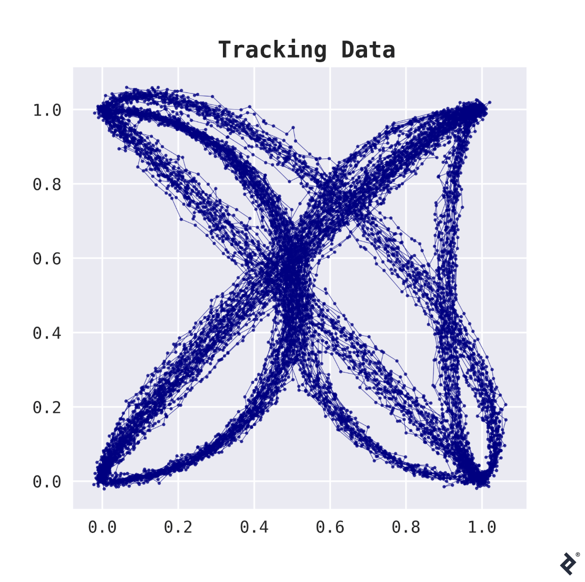
The dataset contains information on 200 tracked shipments. For every tracked shipment, there is a list of (x,y)-coordinates of all locations where the package was spotted, which is typically somewhere between 20 and 50 observations. The plot below shows how this data looks.

This data looks like trouble—two different flavors of trouble, actually.
The first problem is that the data we’re dealing with is high-dimensional. For example, if every package was spotted at 50 locations, our data would have 100 dimensions—sounds like a lot, compared to the 200 samples at your disposition.
The second problem: Different shipment routes actually have a different number of observations, so we cannot simply stack the lists with coordinates to represent the data in a tabular form (and even if they had, that still wouldn’t really make sense).
The merchant is impatiently drumming the table with his fingers, and the data scientist is trying hard not to show any signs of panic.
This is where distance matrices and embeddings will come in handy. We just need to find a way to compare two shipment routes. Fréchet distance seems to be a reasonable choice. With a distance, we can compute a distance matrix.
Note: This step might take a while. We need to compute $O(n^2)$ distances with each distance having $O(k^2)$ iterations, where $n$ is the number of samples and $k$ is the number of observations in one sample. Writing a distance function efficiently is key. For example, in Python, you could use numba to accelerate this computation manyfold.
Visualizing Embeddings
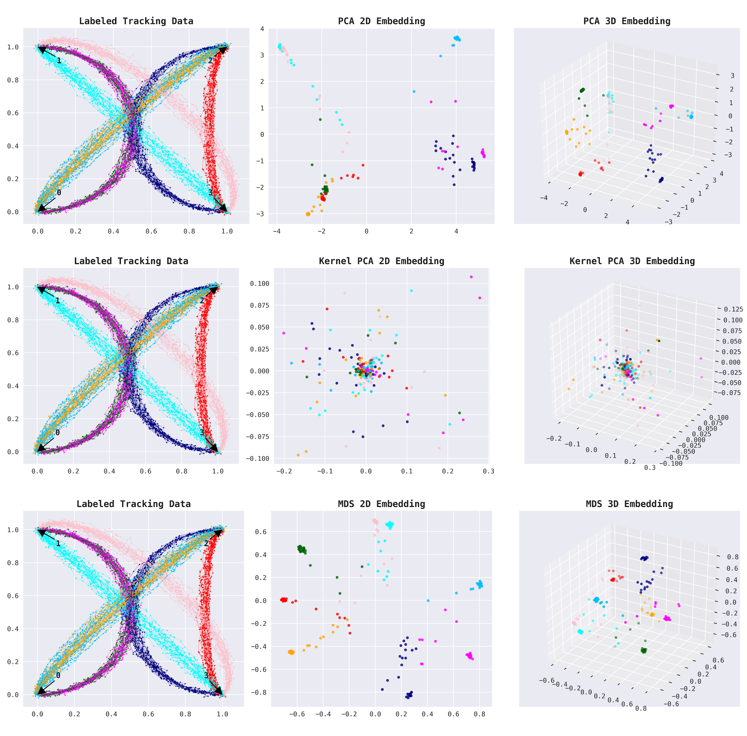
Now, we can use an embedding to reduce the number of dimensions from 200 to just a few. We can clearly see that there are only a few trade routes, so we may hope to find a good representation of the data even in two or three dimensions. We will use embeddings we discussed earlier: PCA, Kernel PCA, and MDS.
On the plots below, you can see the labeled route data (given for the sake of demonstration) and its representation by an embedding in 2D and 3D (from left to right). The labeled data marks four trade posts connected by six trade routes. Two of the six trade routes are bidirectional, which makes eight shipment groups in total (6+2). As you can see, we got a pretty clear separation of all the eight shipment groups with 3D embeddings.

This is a good start.
Embeddings in a Model Pipeline
Now, we are ready to train an embedding. Although MDS showed the best results, it is rather slow; also, scikit-learn’s implementation does not support out-of-sample transformation. It’s not a problem for research but it can be for production, so we will use Kernel PCA instead. For Kernel PCA, we should not forget to apply a radial kernel to the distance matrix beforehand.
How do you select the number of output dimensions? The analysis showed that even 3D works okay. Just to be on the safe side and not leave out any important information, let’s set the embedding output to 10D. For the best performance, the number of output dimensions can be set as a model hyper-parameter and then tuned by cross-validation.
So, we will have 10 numerical features that we can use as an input for pretty much any classification model. How about one linear and one non-linear model: say, Logistic Regression and Gradient Boosting? For comparison, let’s also use these two models with a full distance matrix as the input. On top of it, let’s test SVM too (SVM is designed to work with a distance matrix directly, so no embedding would be required).
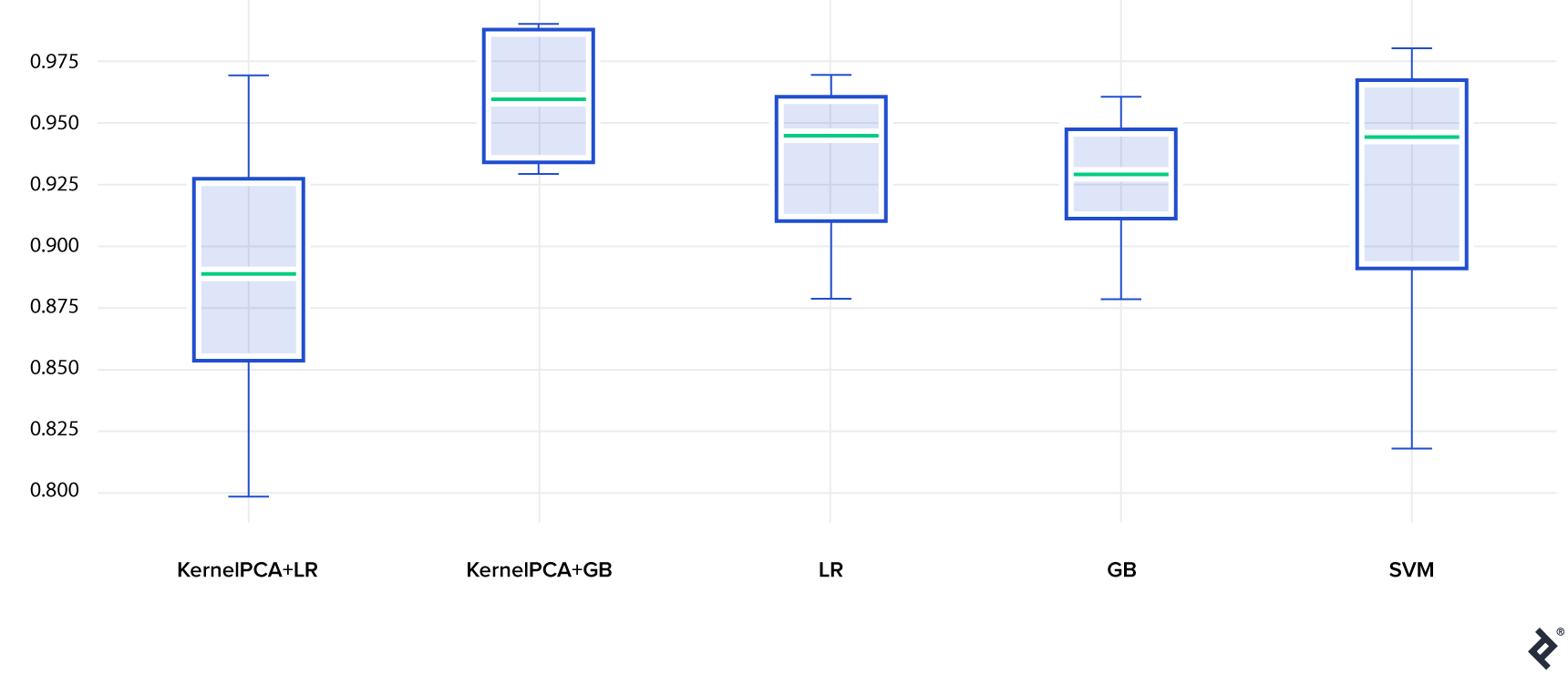
The model accuracy on the test set is shown below (10 train and test datasets were generated so we could estimate the variance of the model):
- Gradient Boosting paired with an embedding (KernelPCA+GB) gets the first place. It outperformed Gradient Boosting with no embedding (GB). Here, Kernel PCA proved to be useful.
- Logistic Regression did okay. What’s interesting is that Logistic Regression with no embedding (LR) did better than with an embedding (KernelPCA+LR). This is not entirely unexpected. Linear models are not very flexible but relatively difficult to overfit. Here, the loss of information caused by an embedding seems to outweigh the benefit of smaller input dimensionality.
- Last but not least, SVM performed well too, although the variance of this model is quite significant.
Model Accuracy

The Python code for this use case is available at GitHub.
Conclusion
We’ve explained what embeddings are and demonstrated how they can be used in conjunction with distance matrices to solve real-world problems. Time for the verdict:
Are embeddings something that a data scientist should use? Let’s take a look at both sides of the story.
Pros & Cons of Using Embeddings
Pros:
- This approach allows us to work with unusual or complex data structures as long as you can define a distance, which—with a certain degree of knowledge, imagination, and luck—you usually can.
- The output is low-dimensional numerical data, which you can easily analyze, cluster, or use as model features for pretty much any machine learning model out there.
Cons:
-
Using this approach, we will necessarily lose some information:
- During the first step, when we replace original data with similarity matrix
- During the second step, when we reduce dimensionality using an embedding
- Depending on data and distance function, computation of a distance matrix may be time-consuming. This may be mitigated by an efficiently written distance function.
- Some embeddings are very sensitive to noise in data. This may be mitigated by additional data cleaning.
- Some embeddings are sensitive to the choice of its hyper-parameters. This may be mitigated by careful analysis or hyper-parameter tuning.
Alternatives: Why Not Use…?
-
Why not just use an embedding directly on data, rather than a distance matrix?
If you know an embedding that can efficiently encode your data directly, by all means, use it. The problem is that it does not always exist.
-
Why not just use clusterization on a distance matrix?
If your only goal is to segment your dataset, it would be totally okay to do so. Some clusterization methods leverage embeddings too (for example, Spectral Clustering). If you’d like to learn more, here is a tutorial on clusterization.
-
Why not just use a distance matrix as features?
The size of a distance matrix is $(n_{samples}, n_{samples})$. Not all models can deal with it efficiently—some may overfit, some may be slow to fit, some may fail to fit altogether. Models with low variance would be a good choice here, such as linear and/or regularized models.
-
Why not just use SVM with a distance matrix?
SVM is a great model, which performed well in our use case. However, there are some caveats. First, if we want to add other features (could be just simple numerical numbers), we won’t be able to do it directly. We’d have to incorporate them into our similarity matrix and potentially lose some valuable information. Second, as good as SVM is, another model may work better for your particular problem.
-
Why not just use deep learning?
It is true, for any problem, you can find a suitable neural network if you search long enough. Keep in mind, though, that the process of finding, training, validating, and deploying this neural network will not necessarily be a simple one. So, as always, use your best judgment.
In One Sentence
Embeddings in conjunction with distance matrices are an incredibly useful tool if you happen to work with complex non-numerical data, especially when you cannot transform your data into a vector space directly and would prefer to have a low-dimensional input for your model.
Understanding the basics
What is an embedding?
An embedding is a low-dimensional representation of data. For example, a world map is a 2D representation of the 3D surface of Earth, and a Discrete Fourier series is a finite-dimensional representation of an infinite-dimensional sound wave.
What is the purpose of embeddings?
An embedding can reduce the number of data dimensions while preserving important internal relationships within the data. For example, a world map preserves relative positions of terrains and oceans.
How are embeddings trained?
Embedding algorithms in ML typically belong to unsupervised learning. They work on unlabeled data but require manually setting hyper-parameters, such as number of output dimensions.
Why are embeddings important?
High-dimensional data can be difficult to analyze, plot, or use to train an ML model. An embedding can reduce the number of dimensions and greatly simplify these tasks for a data scientist.
Do embeddings work with non-numerical data?
Some embeddings are specifically designed to work with non-numerical data. For example, the famous embedding word2vec converts words into vectors. This article shows how embeddings can work with non-numerical data in very general settings.
Yaroslav Kopotilov
Belgrade, Serbia
Member since April 9, 2020
About the author
Yaroslav is a data scientist with experience in business analysis, predictive modeling, data visualization, data orchestration, and deployment.
Expertise
PREVIOUSLY AT


