Tree Kernels: Quantifying Similarity Among Tree-structured Data
Today, a massive amount of data is available in the form of networks or graphs. For example, the World Wide Web, with its web pages and hyperlinks, social networks, semantic networks, biological networks, citation networks for scientific literature, and so on.
A tree is a special type of graph, and is naturally suited to represent many types of data. The analysis of trees is an important field in computer and data science. In this article, we will look at the analysis of the link structure in trees. In particular, we will focus on tree kernels, a method for comparing tree graphs to each other, allowing us to get quantifiable measurements of their similarities or differences. This an important process for many modern applications such as classification and data analysis.
Dino (BCS) has 6+ years in software development, specializing in back-end and security work using Java, Elasticsearch, .NET, and Python.
PREVIOUSLY AT

A network or graph is a type of structured data in the form of nodes, with relationships between them described by links, or edges. Nodes and edges in a graph may have several attributes that may be numerical or categorical, or even more complex.
Today, a massive amount of data is available in the form of networks or graphs. For example, the World Wide Web, with its web pages and hyperlinks, social networks, semantic networks, biological networks, citation networks for scientific literature, and so on.
A tree is a special type of graph, and is naturally suited to represent many types of data. The analysis of trees is an important field in computer and data science. In this article, we will look at the analysis of the link structure in trees. In particular, we will focus on tree kernels, a method for comparing tree graphs to each other, allowing us to get quantifiable measurements of their similarities or differences. This an important process for many modern applications such as classification and data analysis.

Unsupervised Classification of Structured Data
Classification is an important component machine learning and data analysis. In general, classification can either be supervised or unsupervised. In supervised classification, the classes are already known, and a classification model is constructed from training data in which the correct classes are already given. Unsupervised classification, by contrast, attempts to identify classes where none are known, grouping data into categories based on some measure of their similarity.
Unsupervised classification can be combined with graph theory to identify groups of similar tree networks. Tree data structures are employed to model objects from several domains. In natural language processing (NLP), for example, parse trees are modelled as ordered, labelled trees. In automated reasoning, many problems are solved by searching, where the search space is represented as a tree whose vertices are associated with search states, and edges represent inference steps. Also, semistructured data, such as HTML and XML documents, can be modelled as ordered, labelled trees.
These domains can be usefully analysed through unsupervised classification techniques. In NLP, classification can be used to automatically group a set of sentences into questions, commands, and statements. Likewise, groups of similar websites can be identified by applying classification methods to their HTML source. In each of these cases, all we need is a way to measure how “similar” two trees are to each other.
The Curse of Dimensionality
Most classification algorithms require that data be transformed into a vectorized form, representing the values of the data’s features in the feature space, so that the data can by analyzed in the feature space using linear algebra. In structured or semistructured data, like trees, the dimensionality of the resultant vectors (that is, the number of features in the feature space) might be quite high, since the feature space must preserve information about the structure.
This may be a significant drawback, considering that many classification techniques are not able to scale effectively with the dimensionality of the input. In other words, their classification power decreases with an increase in the dimensionality of the input. This problem is known as the curse of dimensionality.
To get an idea of the reason for this degradation of performance, consider a space X of dimension d. Suppose that X contains a set of points uniformly distributed. If the number of dimensions of X increases, the number of points necessary to keep the same density must increase exponentially. In other words, the more the dimensions of the input, the more likely that that data is sparse. In general, a sparse dataset does not give enough information to build a good classifier because correlations between data elements are too weak for algorithms to detect.
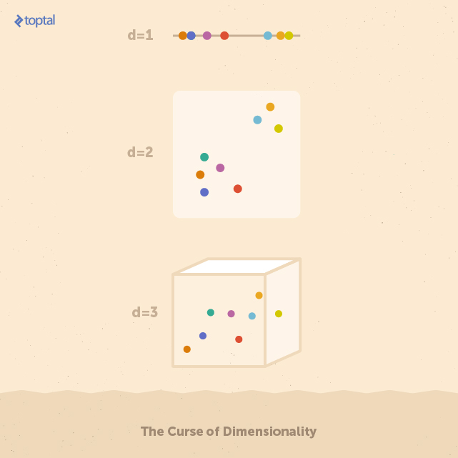
Each feature space above contains eight data points. On the one-dimensional space, it’s easy to identify a group of five points on the left, and three on the right. Stretching these points over higher numbers of features (i.e. dimensions) makes it more difficult to find these groups. In real applications, feature spaces can easily have hundreds of dimensions.
A vectorized representation for structured data is appropriate when information about the domain can be effectively used to select a manageable set of features. When such information is not available, it’s desirable to make use of techniques that can handle structured data directly, without performing operations in the vector space.
Kernel Methods
Kernel methods avoid the need to convert data into vector form. The only information they require is a measurement of the similarity of each pair of items in a data set. This measurement is called a kernel, and the function for determining it is called the kernel function. Kernel methods look for linear relations in the feature space. Functionally, they are equivalent to taking the dot product of two data points in the feature space, and indeed feature design may still be a useful step in kernel function design. However, kernel methods methods avoid directly operating on the feature space since it can be shown that it’s possible to replace the dot product with a kernel function, as long as the kernel function is a symmetric, positive semidefinite function which can take as inputs the data in its original space.
The advantage of using kernel functions is thus that a huge feature space can be analyzed with a computational complexity not dependent on the size of the feature space, but on the complexity of the kernel function, which means that kernel methods do not to suffer the curse of dimensionality.
If we consider a finite dataset composed of n examples, we can get a complete representation of similarities within the data by generating a kernel matrix whose size is always n × n. This matrix is independent of the size of each individual example. This property is useful when a small dataset of examples with a large feature space is to be analyzed.
In general, kernel methods are based on a different answer to the question of data representation. Instead of mapping the input points into a feature space, the data is represented via pairwise comparisons in a kernel matrix K, and all relevant analysis can be performed over the kernel matrix.
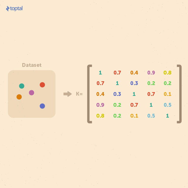
Many data mining methods can be kernelized. To classify tree-structured data instances with kernel methods, such as with support vector machines, it suffices to define a valid (symmetric positive definite) kernel function k : T × T → R, also referred to as a tree kernel. In the design of practically useful tree kernels, one would require them to be computable in polynomial time over the size of the tree, and to be able to detect isomorphic graphs. Such tree kernels are called complete tree kernels.
Tree Kernels
Now, let’s introduce some useful tree kernels for measuring the similarity of trees. The main idea is to calculate the kernel for each pair of trees in the data set in order to build a kernel matrix, which can then be used for classifying sets of trees.
String Kernel
First, we will start with a short introduction to string kernels, which will help us to introduce another kernel method that is based on converting trees into strings.
Let’s define numy(s) as the number of occurrences of a substring y in a string s, with |s| denoting the length of string. The string kernel that we shall describe here is defined as:
Kstring(S1, S2) = Σs∈F nums(S1)nums(S2)ws
Where F is the set of substrings that occur in both S1 and S2, and the parameter ws serves as a weight parameter (for example, to emphasize important substrings). As we can see, this kernel gives a higher value to a pair of strings when they share many common substrings.
Tree Kernel Based on Converting Trees into Strings
We can use this string kernel to build a tree kernel. The idea behind this kernel is to convert two trees into two strings in a systematic way that encodes the tree’s structure, and then apply the above string kernel to them.
We convert the two trees into two strings as follows:
Let T denote one of the target trees, and label(ns) the string label of node ns in T. tag(ns) denotes the string representation of the subtree of T rooted at ns. So if nroot is the root node of T, tag(nroot) is the string representation of the entire tree T.
Next, let string(T) = tag(nroot) denote the string representation of T. We will recursively apply the following steps in a bottom-up fashion to obtain string(T):
- If the node ns is a leaf, let tag(ns) = “[” + label(ns) + “]” (where + here is the string concatenation operator).
- If the node ns is not a leaf and has c children n1, n2, … , nc, sort tag(n1), tag(n2), … , tag(nc) in lexical order to obtain tag(n1*), tag(n2*), … , tag(nc*), and let tag(ns) = “[” + label(ns) + tag(n1*) + tag(n2*) + … + tag(nc*) + “]”.
The figure below, shows an example of this tree-to-string conversion. The result is a string starting with an opening delimiter such as “[” and ending with its closing counterpart, “]”, with each nested pair of delimiters corresponding to a subtree rooted at a particular node.
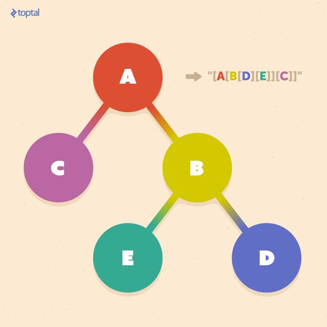
Now we can apply the above conversion to two trees, T1 and T2, to obtain two strings S1 and S2. From there, we can simply apply the string kernel described above.
The tree kernel between T1 and T2 via two strings S1 and S2 can now be given as:
Ktree(T1, T2) = Kstring( string(T1), string(T2) ) = Kstring(S1, S2) = Σs∈F nums(S1)nums(S2)ws
In most applications, the weight parameter becomes w|s|, weighting a substring based on its length |s|. Typical weighting methods for w|s| are:
- constant weighting (w|s| = 1)
- k-spectrum weighting (w|s| = 1 if |s| = k, and w|s| = 0 otherwise)
- exponential weighting (w|s| = λ|s| where 0 ≤ λ ≤ 1 is a decaying rate)
To compute the kernel, it’s sufficient to determine all of the common substrings F, and to count the number of times they occur in S1 and S2. This additional step of finding common substrings is a well-studied problem, and can be accomplished in O(|S1| + |S2|), employing suffix trees or suffix arrays. If we assume that the maximum number of letters (bits, bytes, or characters, for example) needed to describe a node’s label is constant, the lengths of the converted strings are |S1| = O(|T1|) and |S2| = O(|T2|). So, the computational complexity of computing the kernel function is O(|T1| + |T2|), which is linear.
Tree Kernel Based on Subpaths
The tree kernel above used a horizontal, or breadth-first, approach to converting trees to strings. While this approach is quite simple, this conversion means it cannot operate on the trees directly in their original form.
This section will define a tree kernel that operates on the vertical structures in trees, allowing the kernel to operate on the tree directly.
A subsection of a path from the root to one of the leaves is called a subpath, and a subpath set is the set of all subpaths included in the tree:
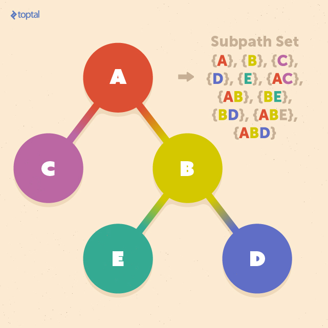
Let us assume that we want to define a tree kernel K(T1, T2) between two trees T1 and T2. By using the subpath set, we can define this tree kernel as:
K(T1, T2) = Σp∈P nump(T1)nump(T2)w|p|
Where nump(T) is the number of of times subpath p occurs in tree T, |p| is the number of nodes in subpath p, and P is the set of all subpaths in T1 and T2. w|p| is the weight, similar to that introduced in the previous section.
Here, we present a simple implementation of this kernel using a depth-first search. Although this algorithm runs in quadratic time, more efficient algorithms exist using suffix trees or suffix arrays, or an extension of the multikey quicksort algorithm, which can achieve linearithmic time ( O(|T1|log|T2|) ) on average:
subpath_track = {}

def generate_subpaths(path, l):
  if l == len(path):
    if tuple(path) not in subpath_track:
      subpath_track[tuple(path)] = 1
    else:
      subpath_track[tuple(path)] += 1
  else:
    index = 0
    while l+index-1 < len(path):
      if tuple(path[index: l+index]) not in subpath_track:
        subpath_track[tuple(path[index: l+index])] = 1
      else:
        subpath_track[tuple(path[index: l+index])] += 1
      index += 1

    generate_subpaths(path, l+1)


def get_subpaths(graph, root, track, path):
  track[root] = True

  if graph.degree(root) == 1:
    generate_subpaths(path, 1)
  else:
    for node in graph.neighbors(root):
      if node not in track:
        get_subpaths(graph, node, track, path + [node, ])


def kernel_subpath(t1, t2, common_track):
  kernel_v = 0
  for p in subpath_track:
    kernel_v += common_track[t1][p]*common_track[t2][p]

  return kernel_v
In this example, we used the weighting parameter w|s| w|p| = 1. This gives all subpaths equal weighting. However, there are many cases when using k-spectrum weighting, or some dynamically assigned weight value, is appropriate.
Mining Websites
Before we wrap up, let’s briefly look at one real-world application of tree classification: categorization of websites. In many data-mining contexts, it is beneficial to know what “type” of website some data comes from. It turns out that pages from different websites can be categorized quite effectively using trees due to similarities in how web pages for similar services are structured.
How do we do that? HTML documents have a logical nested structure, which is very much like a tree. Each document contains one root element, with additional elements nested inside. Nested elements in an HTML tag are logically equivalent to child nodes of that tag:

Let’s take a look at some code that can convert an HTML document into a tree:
def html_to_dom_tree(root):
  node_id = 1
  q = deque()
  graph = nx.Graph()

  q.appendleft({'element': root, "root_id": node_id})
  while len(q):
    node = q.pop()

    if node and node['element'].name == "body":
      graph.add_node(node_id, element=node['element'].name)
      node_id += 1

    root_id = node['root_id']
    labels[root_id] = node['element'].name

    for t in node['element'].contents:
      if t and t.name:
        graph.add_node(node_id, element=t.name)
        graph.add_edge(root_id, node_id)
        q.appendleft({"element": t, "root_id": node_id})
        node_id += 1

  return graph
This will produce a tree data structure that might look something like this:
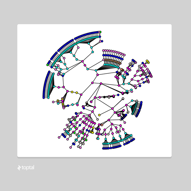
The implementation above makes use of a couple of helpful Python libraries: NetworkX, for working with complex graph structures, and Beautiful Soup, for pulling data from the web and manipulating documents.
Calling html_to_dom_tree(soup.find("body")) will return a NetworkX graph object rooted at the <body> element of the webpage.
Say we want to find groups in a set of 1,000 website homepages. By converting each homepage into a tree like this, we can compare each, for example by using the subpath tree kernel given in the previous section. With these measurements of similarity, we could find that, for example, e-commerce sites, news sites, blogs, and educational sites are easily identified by their similarity to each other.
Conclusion
In this article, we introduced methods for comparing tree-structured data elements to each other, and showed how to apply kernel methods to trees to get a quantifiable measurement of their similarity. Kernel methods have proven to be an excellent choice when operating in high-dimensional spaces, a common situation when working with tree structures. These techniques set the stage for further analysis of large sets of trees, using well-studied methods that operate over the kernel matrix.
Tree structures are encountered in many real-word areas like XML and HTML documents, chemical compounds, natural language processing, or certain types of users behavior. As demonstrated in the example of constructing trees from HTML, these techniques empower us to perform meaningful analysis in these domains.
Dino Causevic
Sarajevo, Federation of Bosnia and Herzegovina, Bosnia and Herzegovina
Member since December 26, 2014
About the author
Dino (BCS) has 6+ years in software development, specializing in back-end and security work using Java, Elasticsearch, .NET, and Python.
PREVIOUSLY AT


