Create Data From Random Noise With Generative Adversarial Networks
Generative adversarial networks, among the most important machine learning breakthroughs of recent times, allow you to generate useful data from random noise. Instead of training one neural network with millions of data points, you let two neural networks contest with each other to figure things out.
In this article, Toptal Freelance Software Engineer Cody Nash gives us an overview of how GANs work and how this class of machine learning algorithms can be used to generate data in data-limited situations.
As a data scientist, Cody has used tools including Python and R to explore and deploy analyses on genetic, healthcare and other data sets.
Expertise
Since I found out about generative adversarial networks (GANs), I’ve been fascinated by them. A GAN is a type of neural network that is able to generate new data from scratch. You can feed it a little bit of random noise as input, and it can produce realistic images of bedrooms, or birds, or whatever it is trained to generate.
One thing all scientists can agree on is that we need more data.
GANs, which can be used to produce new data in data-limited situations, can prove to be really useful. Data can sometimes be difficult and expensive and time-consuming to generate. To be useful, though, the new data has to be realistic enough that whatever insights we obtain from the generated data still applies to real data. If you’re training a cat to hunt mice, and you’re using fake mice, you’d better make sure that the fake mice actually look like mice.
Another way of thinking about it is the GANs are discovering structure in the data that allows them to make realistic data. This can be useful if we can’t see that structure on our own or can’t pull it out with other methods.
In this article, you will learn how GANs can be used to generate new data. To keep this tutorial realistic, we will use the credit card fraud detection dataset from Kaggle.
In my experiments, I tried to use this dataset to see if I can get a GAN to create data realistic enough to help us detect fraudulent cases. This dataset highlights the limited data issue: Out of 285,000 transactions, only 492 are fraud. 492 cases of fraud is not a large dataset to train on, especially when it comes to machine learning tasks where people like to have datasets several orders of magnitude larger. Although the results of my experiment were not amazing, I did learn a lot about GANs along the way that I’m happy to share.
Before You Start
Before we delve into this realm of GANs, if you want to quickly brush up on your machine learning or deep learning skills, you can take a look at these two related blog posts:
- An Introduction to Machine Learning Theory and Its Application: A Visual Tutorial with Examples
- A Deep Learning Tutorial: From Perceptrons to Deep Networks
Why GANs?
Generative adversarial networks (GANs) are a neural network architecture that has shown impressive improvements over previous generative methods, such as variational auto-encoders or restricted boltzman machines. GANs have been able to generate more realistic images (e.g., DCGAN), enable style transfer between images (see here and here), generate images from text descriptions (StackGAN), and learn from smaller datasets via semi-supervised learning. Because of these achievements, they are generating a lot of interest in both the academic and commercial sectors.
The Director of AI Research at Facebook, Yann LeCunn, has even called them the most exciting development in machine learning in the last decade.
The Basics
Think about how you learn. You try something, you get some feedback. You adjust your strategy and try again.
The feedback may come in the form of criticism, or pain, or profit. It may come from your own judgment of how well you did. Often, the most useful feedback is the feedback that comes from another person, because it isn’t just a number or sensation, but an intelligent assessment of how well you performed the task.
When a computer is trained for a task, the human usually provides the feedback in the form of adjusted parameters or algorithms. This works well when the task is well defined, such as learning to multiply two numbers. You can easily and exactly tell the computer how it was wrong.
With a more complicated task, such as creating an image of dog, it becomes more difficult to provide feedback. Is the image blurry, does it look more like a cat, or does it look like anything at all? Complex statistics could be implemented, but it would be hard to capture all the details that make an image seem real.
A human can give some estimation, because we have lots of experience evaluating visual input, but we are relatively slow and our evaluations can be highly subjective. We could instead train a neural network to learn the task of discriminating between real and generated images.
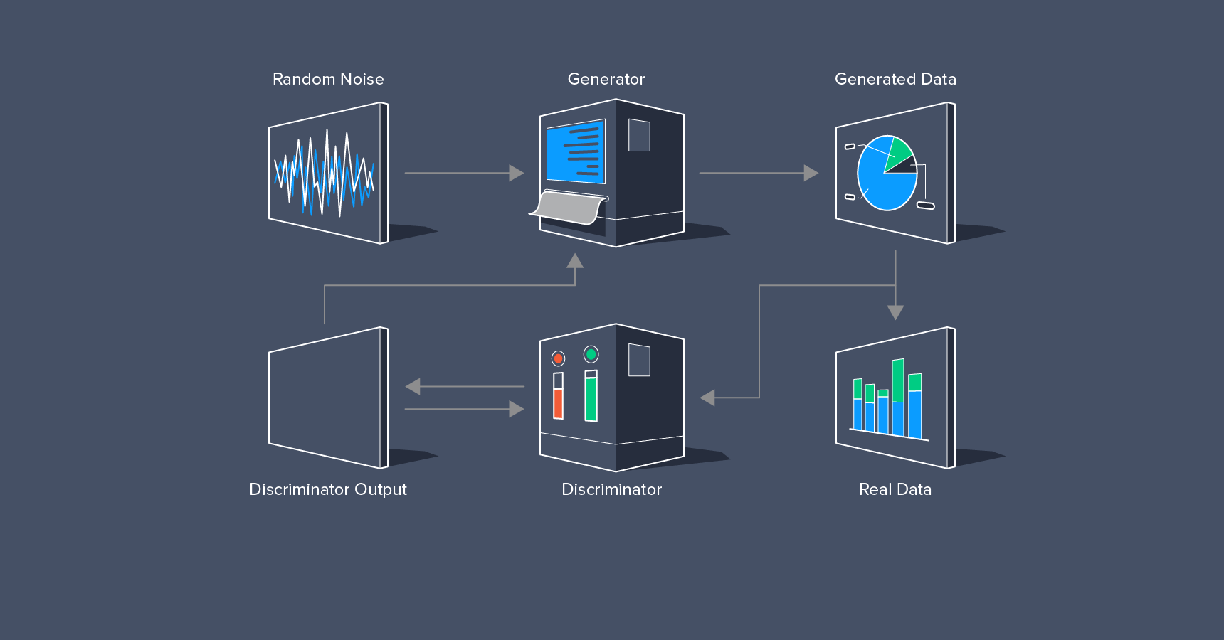
Then, by letting the image generator (also a neural network) and the discriminator take turns learning from each other, they can improve over time. These two networks, playing this game, are a generative adversarial network.
You can hear the inventor of GANs, Ian Goodfellow, talk about how an argument at a bar on this topic led to a feverish night of coding that resulted in the first GAN. And yes, he does acknowledge the bar in his paper. You can learn more about GANs from Ian Goodfellow’s blog on this topic.
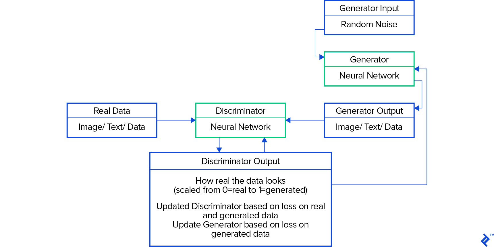
There are a number of challenges when working with GANs. Training a single neural network can be difficult due to the number of choices involved: Architecture, activation functions, optimization method, learning rate, and dropout rate, to name just a few.
GANs double all of those choices and add new complexities. Both the generator and the discriminator may forget tricks they used earlier in their training. This can lead to the two networks getting caught in a stable cycle of solutions that do not improve over time. One network may overpower the other network, such that neither can learn anymore. Or, the generator may not explore much of the possible solution space, only enough of it to find realistic solutions. This last situation is known as mode collapse.
Mode collapse is when the generator only learns a small subset of the possible realistic modes. For instance, if the task is to generate images of dogs, the generator could learn to create only images of small brown dogs. The generator would have missed all of the other modes consisting of dogs of other sizes or colors.
Many strategies have been implemented to address this, including batch normalization, adding labels in the training data, or by changing the way the discriminator judges the generated data.
People have noted that adding labels to the data—that is, to break it up into categories, almost always improves the performance of GANs. Instead of learning to generate images of pets in general, it should be easier to generate images of cats, dogs, fish, and ferrets, for example.
Perhaps the most significant breakthroughs in GAN development have come in terms of changing how the discriminator evaluates data, so let’s take a closer look at that.
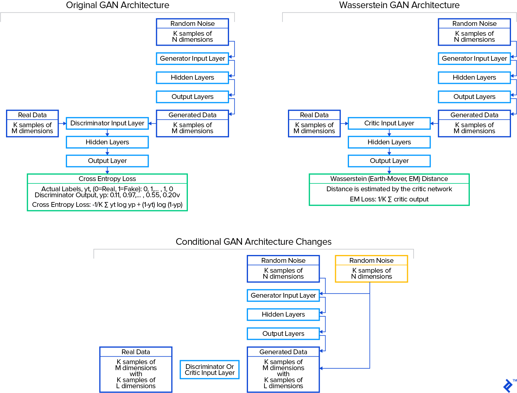
In the original formulation of GANs in 2014 by Goodfellow et al., the discriminator generates an estimate of the probability that a given image was real or generated. The discriminator would be supplied a set of images that consisted of both real and generated images and it would generate an estimate for each of these inputs. The error between the discriminator output and the actual labels would then be measured by cross-entropy loss. Cross-entropy loss can be equated to the Jensen-Shannon distance metric, and it was shown in early 2017 by Arjovsky et al. that this metric would fail in some cases and not point in the right direction in other cases. This group showed that the Wasserstein distance metric (also known as the earth mover or EM distance) worked and worked better in many more cases.
The cross-entropy loss is a measure of how accurately the discriminator identified real and generated images. The Wasserstein metric instead looks at the distribution of each variable (i.e., each color of each pixel) in the real and generated images, and determines how far apart the distributions are for real and generated data. The Wasserstein metric looks at how much effort, in terms of mass times distance, it would take to push the generated distribution into the shape of the real distribution, hence the alternate name “earth mover distance.” Because the Wasserstein metric is no longer evaluating whether an image is real or not, but is instead providing criticism of how far the generated images are from the real images, the “discriminator” network is referred to as the “critic” network in the Wasserstein architecture.
For a slightly more comprehensive exploration of GANs, in this article, we will explore four different architectures:
- GAN: The original (“vanilla”) GAN
- CGAN: A conditional version of the original GAN that makes use of class labels
- WGAN: The Wasserstein GAN (with gradient-penalty)
- WCGAN: A conditional version of the Wasserstein GAN
But let’s glance at our dataset first.
A Look at Credit Card Fraud Data
We will be working with the credit card fraud detection dataset from Kaggle.
The dataset consists of ~285,000 transactions, of which only 492 are fraudulent. The data consists of 31 features: “time,” “amount,” “class,” and 28 additional, anonymized features. The class feature is the label indicating whether a transaction is fraudulent or not, with 0 indicating normal and 1 indicating fraud. All of the data is numeric and continuous (except the label). The data set has no missing values. The dataset is already in pretty good shape to start with, but I’ll do a little more cleaning, mostly just adjusting the means of all the features to zero and the standard deviations to one. I’ve described my cleaning process more in the notebook here. For now I’ll just show the end result:
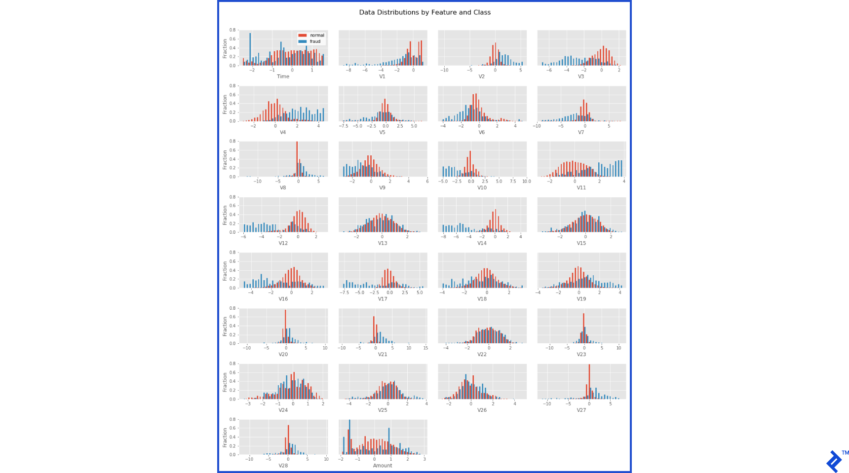
One can readily spot differences between the normal and fraud data in these distributions, but there is also a lot of overlap. We can apply one of the faster and more powerful machine learning algorithms to identify the most useful features for identifying fraud. This algorithm, xgboost, is a gradient-boosted decision tree algorithm. We’ll train it on 70% of the dataset, and test it on the remaining 30%. We can set up the algorithm to continue until it doesn’t improve recall (the fraction of fraud samples detected) on the test dataset. This achieves 76% recall on the test set, which clearly leaves room for improvement. It does achieve a precision of 94%, meaning of that only 6% of the predicted fraud cases were actually normal transactions. From this analysis, we also get a list of features sorted by their utility in detecting fraud. We can use the most important features to help visualize our results later on.
Again, if we had more fraud data, we might be able to detect it better. That is, we could achieve a higher recall. We will now try to generate new, realistic fraud data using GANs to help us detect actual fraud.
Generating New Credit Card Data with GANs
To apply various GAN architectures to this dataset, I’m going to make use of GAN-Sandbox, which has a number of popular GAN architectures implemented in Python using the Keras library and a TensorFlow back-end. All of my results are available as a Jupyter notebook here. All of the necessary libraries are included in the Kaggle/Python Docker image, if you need an easy setup.
The examples in GAN-Sandbox are set up for image processing. The generator produces a 2D image with 3 color channels for each pixel, and the discriminator/critic is configured to evaluate such data. Convolutional transformations are utilized between layers of the networks to take advantage of the spatial structure of image data. Each neuron in a convolutional layer only works with a small group of inputs and outputs (e.g., adjacent pixels in an image) to allow learning of spatial relationships. Our credit card dataset lacks any spatial structure among the variables, so I’ve converted the convolutional networks to networks with densely connected layers. The neurons in densely connected layers are connected to every input and output of the layer, allowing the network to learn its own relationships among the features. I’ll use this setup for each of the architectures.
The first GAN I’ll evaluate pits the generator network against the discriminator network, making use of the cross-entropy loss from the discriminator to train the networks. This is the original, “vanilla” GAN architecture. The second GAN I’ll evaluate adds class labels to the data in the manner of a conditional GAN (CGAN). This GAN has one more variable in the data, the class label. The third GAN will use the Wasserstein distance metric to train the networks (WGAN), and the last one will use the class labels and the Wasserstein distance metric (WCGAN).
We’ll train the various GANs using a training dataset that consists of all 492 fraudulent transactions. We can add classes to the fraud dataset to facilitate the conditional GAN architectures. I’ve explored a few different clustering methods in the notebook and went with a KMeans classification that sorts the fraud data into 2 classes.
I’ll train each GAN for 5000 rounds and examine the results along the way. In Figure 4, we can see the actual fraud data and the generated fraud data from the different GAN architectures as training progresses. We can see the actual fraud data divided into the 2 KMeans classes, plotted with the 2 dimensions that best discriminate these two classes (features V10 and V17 from the PCA transformed features). The two GANs that do not make use of class information, the GAN and WGAN, have their generated output all as one class. The conditional architectures, the CGAN and WCGAN, show their generated data by class. At step 0, all of the generated data shows the normal distribution of the random input fed to the generators.
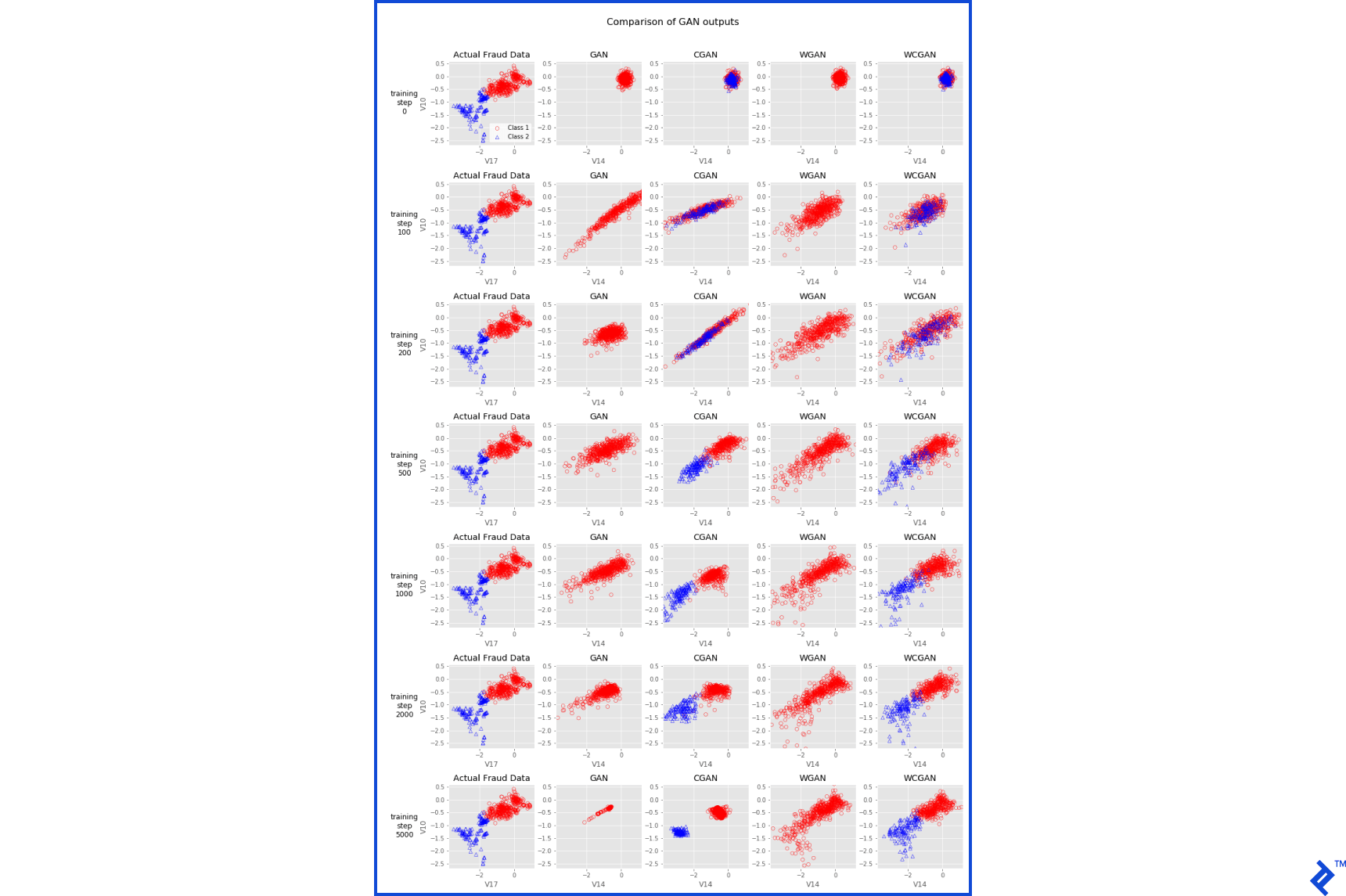
We can see that the original GAN architecture starts to learn the shape and range of the actual data, but then collapses towards a small distribution. This is the mode collapse discussed earlier. The generator has learned a small range of data that the discriminator has a hard time detecting as fake. The CGAN architecture does a little better, spreading out and approaching the distributions of each class of fraud data, but then mode collapse sets in, as can be seen at step 5000.
The WGAN does not experience the mode collapse exhibited by the GAN and CGAN architectures. Even without class information, it begins to assume the non-normal distribution of the actual fraud data. The WCGAN architecture performs similarly and is able to generate the separate classes of data.
We can evaluate how realistic the data looks using the same xgboost algorithm used earlier for fraud detection. It’s fast and powerful and works off-the-shelf without much tuning. We’ll train the xgboost classifier using half the actual fraud data (246 samples) and an equal number of GAN-generated examples. Then we’ll test the xgboost classifier using the other half of the actual fraud data and a different set of 246 GAN generated examples. This orthogonal method (in the experimental sense) will give us some indication of how successful the generator is in producing realistic data. With perfectly realistic generated data, the xgboost algorithm should achieve an accuracy of 0.50 (50%)—in other words, it is no better than guessing.
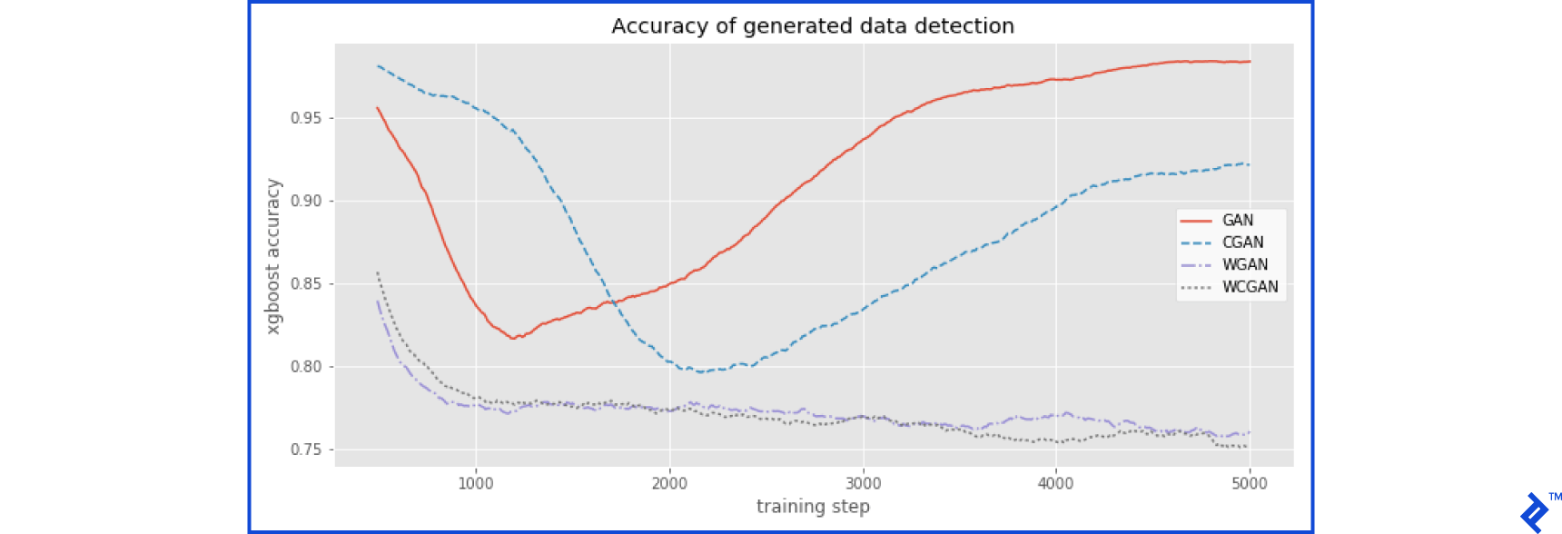
We can see the xgboost accuracy on the GAN generated data decreasing at first, and then increasing after training step 1000 as mode collapse sets in. The CGAN architecture achieves somewhat more realistic data after 2000 steps, but then mode collapse sets in for this network as well. The WGAN and WCGAN architectures achieve more realistic data faster, and continue to learn as the training progresses. The WCGAN does not appear to have much of an edge over the WGAN, suggesting that these created classes may not be useful for the Wasserstein GAN architectures.
You can learn more about the WGAN architecture from here and here.
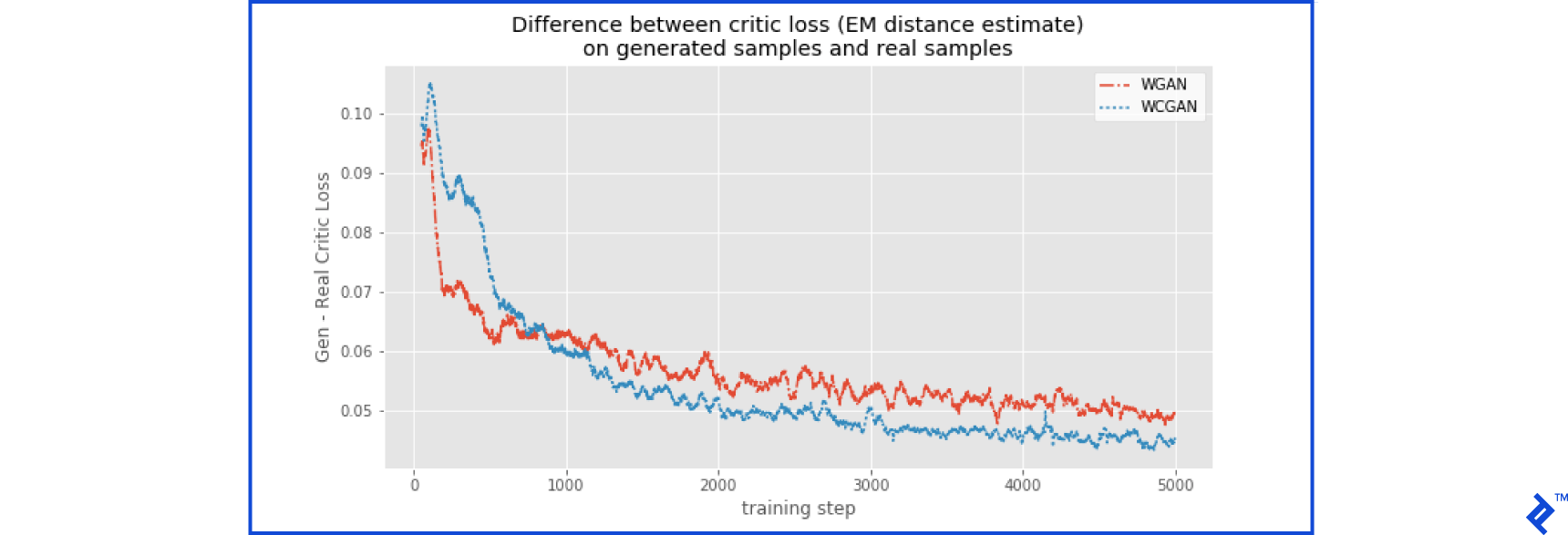
The critic network in the WGAN and WCGAN architectures is learning to calculate the Wasserstein (Earth-mover, EM) distance between a given dataset and the actual fraud data. Ideally, it will measure a distance of close to zero for a sample of actual fraud data. The critic, however, is in the process of learning how to perform this calculation. As long it as measures a larger distance for generated data than for real data, the network can improve. We can watch how the difference between Wasserstein distances for generated and real data changes over the course of training. If it plateaus, then further training may not help. We can see in figure 6 that there appears to be further improvement to be had for both the WGAN and WCGAN on this dataset.
What Did We Learn?
Now we can test if we are able to generate new fraud data realistic enough to help us detect actual fraud data. We can take the trained generator that achieved the lowest accuracy score and use that to generate data. For our basic training set, we’ll use 70% of the non-fraud data (199,020 cases) and 100 cases of the fraud data (~20% of the fraud data). Then we’ll try adding different amounts of real or generated fraud data to this training set, up to 344 cases (70% of the fraud data). For the test set, we’ll use the other 30% of the non-fraud cases (85,295 cases) and fraud cases (148 cases). We can try adding generated data from an untrained GAN and from the best trained GAN to test if the generated data is any better than random noise. From our tests, it appears that our best architecture was the WCGAN at training step 4800, where it achieved an xgboost accuracy of 70% (remember, ideally, accuracy would be 50%). So we’ll use this architecture to generate new fraud data.
We can see in figure 7 that recall (the fraction of actual fraud samples accurately identified in the test set) does not increase as we use more generated fraud data for training. The xgboost classifier is able to retain all the information it used to identify fraud from the 100 real cases and not get confused by the additional generated data, even when picking them out of hundreds of thousands of normal cases. The generated data from the untrained WCGAN doesn’t help or hurt, unsurprisingly. But the generated data from the trained WCGAN doesn’t help either. It appears the data isn’t realistic enough. We can see in figure 7 that when actual fraud data is used to supplement the training set, the recall significantly increases. If the WCGAN had just learned to duplicate the training examples, without getting creative at all, it could have achieved higher recall rates as we see with the real data.

To Infinity and Beyond
While we were unable to generate credit card fraud data realistic enough to help us detect actual fraud, we have barely scratched the surface with these methods. We could train longer, with larger networks, and tune parameters for the architectures we tried in this article. The trends in xgboost accuracy and discriminator loss suggest more training will help the WGAN and WCGAN architectures. Another option is to revisit the data cleaning we performed, perhaps engineer some new variables or change if and how we address skewness in features. Perhaps different classification schemes of the fraud data would help.
We could also try other GAN architectures. The DRAGAN has theoretical and experimental evidence showing that it trains faster and more stably than the Wasserstein GANs. We could integrate methods that make use of semi-supervised learning, which have shown promise in learning from limited training sets (see “Improved Techniques for Training GANs”). We could try an architecture that gives us human-understandable models, so we might be able to understand the structure of the data better (see InfoGAN).
We should also keep an eye out for new developments in the field, and last but certainly not least, we can work on creating our own innovations in this rapidly developing space.
You can find all of the relevant code for this article in this GitHub repository.
Understanding the basics
What is a GAN?
A GAN is a machine learning algorithm where one neural network generates the data while another one determines if the output looks real. The two networks contest against each other to improve the realism of the generated data.
Bratislava, Bratislava Region, Slovakia
Member since May 8, 2017
About the author
As a data scientist, Cody has used tools including Python and R to explore and deploy analyses on genetic, healthcare and other data sets.

