
A Deep Learning Tutorial: From Perceptrons to Deep Networks
The recent resurgence in Artificial Intelligence has been powered in no small part by a new trend in machine learning, known as “Deep Learning”. In this article, I’ll introduce you to the key concepts and algorithms behind Deep Learning, beginning with the simplest building block.

The recent resurgence in Artificial Intelligence has been powered in no small part by a new trend in machine learning, known as “Deep Learning”. In this article, I’ll introduce you to the key concepts and algorithms behind Deep Learning, beginning with the simplest building block.

Ivan is an enthusiastic senior developer with an entrepreneurial spirit. His primary focuses are in Java, JavaScript and Machine Learning.
Expertise
Previously At

In recent years, there’s been a resurgence in the field of Artificial Intelligence. It’s spread beyond the academic world with major players like Google, Microsoft, and Facebook creating their own research teams and making some impressive acquisitions.
Some this can be attributed to the abundance of raw data generated by social network users, much of which needs to be analyzed, the rise of advanced data science solutions, as well as to the cheap computational power available via GPGPUs.
But beyond these phenomena, this resurgence has been powered in no small part by a new trend in AI, specifically in machine learning, known as “Deep Learning”. In this tutorial, I’ll introduce you to the key concepts and algorithms behind deep learning, beginning with the simplest unit of composition and building to the concepts of machine learning in Java.
(For full disclosure: I’m also the author of a Java deep learning library, available here, and the examples in this article are implemented using the above library. If you like it, you can support it by giving it a star on GitHub, for which I would be grateful. Usage instructions are available on the homepage.)
A Thirty Second Tutorial on Machine Learning
In case you’re not familiar, check out this introduction to machine learning:
The general procedure is as follows:
- We have some algorithm that’s given a handful of labeled examples, say 10 images of dogs with the label 1 (“Dog”) and 10 images of other things with the label 0 (“Not dog”)—note that we’re mainly sticking to supervised, binary classification for this post.
- The algorithm “learns” to identify images of dogs and, when fed a new image, hopes to produce the correct label (1 if it’s an image of a dog, and 0 otherwise).
This setting is incredibly general: your data could be symptoms and your labels illnesses; or your data could be images of handwritten characters and your labels the actual characters they represent.
Perceptrons: Early Deep Learning Algorithms
One of the earliest supervised training algorithms is that of the perceptron, a basic neural network building block.
Say we have n points in the plane, labeled ‘0’ and ‘1’. We’re given a new point and we want to guess its label (this is akin to the “Dog” and “Not dog” scenario above). How do we do it?
One approach might be to look at the closest neighbor and return that point’s label. But a slightly more intelligent way of going about it would be to pick a line that best separates the labeled data and use that as your classifier.

In this case, each piece of input data would be represented as a vector x = (x_1, x_2) and our function would be something like “‘0’ if below the line, ‘1’ if above”.
To represent this mathematically, let our separator be defined by a vector of weights w and a vertical offset (or bias) b. Then, our function would combine the inputs and weights with a weighted sum transfer function:

The result of this transfer function would then be fed into an activation function to produce a labeling. In the example above, our activation function was a threshold cutoff (e.g., 1 if greater than some value):

Training the Perceptron
The training of the perceptron consists of feeding it multiple training samples and calculating the output for each of them. After each sample, the weights w are adjusted in such a way so as to minimize the output error, defined as the difference between the desired (target) and the actual outputs. There are other error functions, like the mean square error, but the basic principle of training remains the same.
Single Perceptron Drawbacks
The single perceptron approach to deep learning has one major drawback: it can only learn linearly separable functions. How major is this drawback? Take XOR, a relatively simple function, and notice that it can’t be classified by a linear separator (notice the failed attempt, below):

To address this problem, we’ll need to use a multilayer perceptron, also known as feedforward neural network: in effect, we’ll compose a bunch of these perceptrons together to create a more powerful mechanism for learning.
Feedforward Neural Networks for Deep Learning
A neural network is really just a composition of perceptrons, connected in different ways and operating on different activation functions.

For starters, we’ll look at the feedforward neural network, which has the following properties:
- An input, output, and one or more hidden layers. The figure above shows a network with a 3-unit input layer, 4-unit hidden layer and an output layer with 2 units (the terms units and neurons are interchangeable).
- Each unit is a single perceptron like the one described above.
- The units of the input layer serve as inputs for the units of the hidden layer, while the hidden layer units are inputs to the output layer.
- Each connection between two neurons has a weight w (similar to the perceptron weights).
- Each unit of layer t is typically connected to every unit of the previous layer t - 1 (although you could disconnect them by setting their weight to 0).
- To process input data, you “clamp” the input vector to the input layer, setting the values of the vector as “outputs” for each of the input units. In this particular case, the network can process a 3-dimensional input vector (because of the 3 input units). For example, if your input vector is [7, 1, 2], then you’d set the output of the top input unit to 7, the middle unit to 1, and so on. These values are then propagated forward to the hidden units using the weighted sum transfer function for each hidden unit (hence the term forward propagation), which in turn calculate their outputs (activation function).
- The output layer calculates it’s outputs in the same way as the hidden layer. The result of the output layer is the output of the network.
Beyond Linearity
What if each of our perceptrons is only allowed to use a linear activation function? Then, the final output of our network will still be some linear function of the inputs, just adjusted with a ton of different weights that it’s collected throughout the network. In other words, a linear composition of a bunch of linear functions is still just a linear function. If we’re restricted to linear activation functions, then the feedforward neural network is no more powerful than the perceptron, no matter how many layers it has.
Because of this, most neural networks use non-linear activation functions like the logistic, tanh, binary or rectifier. Without them the network can only learn functions which are linear combinations of its inputs.
Training Perceptrons
The most common deep learning algorithm for supervised training of the multilayer perceptrons is known as backpropagation. The basic procedure:
- A training sample is presented and propagated forward through the network.
-
The output error is calculated, typically the mean squared error:
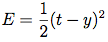
Where t is the target value and y is the actual network output. Other error calculations are also acceptable, but the MSE is a good choice.
-
Network error is minimized using a method called stochastic gradient descent.

Gradient descent is universal, but in the case of neural networks, this would be a graph of the training error as a function of the input parameters. The optimal value for each weight is that at which the error achieves a global minimum. During the training phase, the weights are updated in small steps (after each training sample or a mini-batch of several samples) in such a way that they are always trying to reach the global minimum—but this is no easy task, as you often end up in local minima, like the one on the right. For example, if the weight has a value of 0.6, it needs to be changed towards 0.4.
This figure represents the simplest case, that in which error depends on a single parameter. However, network error depends on every network weight and the error function is much, much more complex.
Thankfully, backpropagation provides a method for updating each weight between two neurons with respect to the output error. The derivation itself is quite complicated, but the weight update for a given node has the following (simple) form:
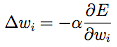
Where E is the output error, and w_i is the weight of input i to the neuron.
Essentially, the goal is to move in the direction of the gradient with respect to weight i. The key term is, of course, the derivative of the error, which isn’t always easy to calculate: how would you find this derivative for a random weight of a random hidden node in the middle of a large network?
The answer: through backpropagation. The errors are first calculated at the output units where the formula is quite simple (based on the difference between the target and predicted values), and then propagated back through the network in a clever fashion, allowing us to efficiently update our weights during training and (hopefully) reach a minimum.


Hidden Layer
The hidden layer is of particular interest. By the universal approximation theorem, a single hidden layer network with a finite number of neurons can be trained to approximate an arbitrarily random function. In other words, a single hidden layer is powerful enough to learn any function. That said, we often learn better in practice with multiple hidden layers (i.e., deeper nets).
The hidden layer is where the network stores it’s internal abstract representation of the training data, similar to the way that a human brain (greatly simplified analogy) has an internal representation of the real world. Going forward in the tutorial, we’ll look at different ways to play around with the hidden layer.
An Example Network
You can see a simple (4-2-3 layer) feedforward neural network that classifies the IRIS dataset implemented in Java here through the testMLPSigmoidBP method. The dataset contains three classes of iris plants with features like sepal length, petal length, etc. The network is provided 50 samples per class. The features are clamped to the input units, while each output unit corresponds to a single class of the dataset: “1/0/0” indicates that the plant is of class Setosa, “0/1/0” indicates Versicolour, and “0/0/1” indicates Virginica). The classification error is 2/150 (i.e., it misclassifies 2 samples out of 150).
The Problem with Large Networks
A neural network can have more than one hidden layer: in that case, the higher layers are “building” new abstractions on top of previous layers. And as we mentioned before, you can often learn better in-practice with larger networks.
However, increasing the number of hidden layers leads to two known issues:
- Vanishing gradients: as we add more and more hidden layers, backpropagation becomes less and less useful in passing information to the lower layers. In effect, as information is passed back, the gradients begin to vanish and become small relative to the weights of the networks.
- Overfitting: perhaps the central problem in machine learning. Briefly, overfitting describes the phenomenon of fitting the training data too closely, maybe with hypotheses that are too complex. In such a case, your learner ends up fitting the training data really well, but will perform much, much more poorly on real examples.
Let’s look at some deep learning algorithms to address these issues.
Autoencoders
Most introductory machine learning classes tend to stop with feedforward neural networks. But the space of possible nets is far richer—so let’s continue.
An autoencoder is typically a feedforward neural network which aims to learn a compressed, distributed representation (encoding) of a dataset.

Conceptually, the network is trained to “recreate” the input, i.e., the input and the target data are the same. In other words: you’re trying to output the same thing you were input, but compressed in some way. This is a confusing approach, so let’s look at an example.
Compressing the Input: Grayscale Images
Say that the training data consists of 28x28 grayscale images and the value of each pixel is clamped to one input layer neuron (i.e., the input layer will have 784 neurons). Then, the output layer would have the same number of units (784) as the input layer and the target value for each output unit would be the grayscale value of one pixel of the image.
The intuition behind this architecture is that the network will not learn a “mapping” between the training data and its labels, but will instead learn the internal structure and features of the data itself. (Because of this, the hidden layer is also called feature detector.) Usually, the number of hidden units is smaller than the input/output layers, which forces the network to learn only the most important features and achieves a dimensionality reduction.
In effect, we want a few small nodes in the middle to really learn the data at a conceptual level, producing a compact representation that in some way captures the core features of our input.
Flu Illness
To further demonstrate autoencoders, let’s look at one more application.
In this case, we’ll use a simple dataset consisting of flu symptoms. If you’re interested, the code for this example can be found in the testAEBackpropagation method.
Here’s how the data set breaks down:
- There are six binary input features.
- The first three are symptoms of the illness. For example, 1 0 0 0 0 0 indicates that this patient has a high temperature, while 0 1 0 0 0 0 indicates coughing, 1 1 0 0 0 0 indicates coughing and high temperature, etc.
- The final three features are “counter” symptoms; when a patient has one of these, it’s less likely that he or she is sick. For example, 0 0 0 1 0 0 indicates that this patient has a flu vaccine. It’s possible to have combinations of the two sets of features: 0 1 0 1 0 0 indicates a vaccines patient with a cough, and so forth.
We’ll consider a patient to be sick when he or she has at least two of the first three features and healthy if he or she has at least two of the second three (with ties breaking in favor of the healthy patients), e.g.:
- 111000, 101000, 110000, 011000, 011100 = sick
- 000111, 001110, 000101, 000011, 000110 = healthy
We’ll train an autoencoder (using backpropagation) with six input and six output units, but only two hidden units.
After several hundred iterations, we observe that when each of the “sick” samples is presented to the machine learning network, one of the two the hidden units (the same unit for each “sick” sample) always exhibits a higher activation value than the other. On the contrary, when a “healthy” sample is presented, the other hidden unit has a higher activation.
Going Back to Machine Learning
Essentially, our two hidden units have learned a compact representation of the flu symptom data set. To see how this relates to learning, we return to the problem of overfitting. By training our net to learn a compact representation of the data, we’re favoring a simpler representation rather than a highly complex hypothesis that overfits the training data.
In a way, by favoring these simpler representations, we’re attempting to learn the data in a truer sense.
Restricted Boltzmann Machines
The next logical step is to look at a Restricted Boltzmann machines (RBM), a generative stochastic neural network that can learn a probability distribution over its set of inputs.

RBMs are composed of a hidden, visible, and bias layer. Unlike the feedforward networks, the connections between the visible and hidden layers are undirected (the values can be propagated in both the visible-to-hidden and hidden-to-visible directions) and fully connected (each unit from a given layer is connected to each unit in the next—if we allowed any unit in any layer to connect to any other layer, then we’d have a Boltzmann (rather than a restricted Boltzmann) machine).
The standard RBM has binary hidden and visible units: that is, the unit activation is 0 or 1 under a Bernoulli distribution, but there are variants with other non-linearities.
While researchers have known about RBMs for some time now, the recent introduction of the contrastive divergence unsupervised training algorithm has renewed interest.
Contrastive Divergence
The single-step contrastive divergence algorithm (CD-1) works like this:
-
Positive phase:
- An input sample v is clamped to the input layer.
- v is propagated to the hidden layer in a similar manner to the feedforward networks. The result of the hidden layer activations is h.
-
Negative phase:
- Propagate h back to the visible layer with result v’ (the connections between the visible and hidden layers are undirected and thus allow movement in both directions).
- Propagate the new v’ back to the hidden layer with activations result h’.
-
Weight update:
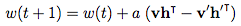
Where a is the learning rate and v, v’, h, h’, and w are vectors.

The intuition behind the algorithm is that the positive phase (h given v) reflects the network’s internal representation of the real world data. Meanwhile, the negative phase represents an attempt to recreate the data based on this internal representation (v’ given h). The main goal is for the generated data to be as close as possible to the real world and this is reflected in the weight update formula.
In other words, the net has some perception of how the input data can be represented, so it tries to reproduce the data based on this perception. If its reproduction isn’t close enough to reality, it makes an adjustment and tries again.
Returning to the Flu
To demonstrate contrastive divergence, we’ll use the same symptoms data set as before. The test network is an RBM with six visible and two hidden units. We’ll train the network using contrastive divergence with the symptoms v clamped to the visible layer. During testing, the symptoms are again presented to the visible layer; then, the data is propagated to the hidden layer. The hidden units represent the sick/healthy state, a very similar architecture to the autoencoder (propagating data from the visible to the hidden layer).
After several hundred iterations, we can observe the same result as with autoencoders: one of the hidden units has a higher activation value when any of the “sick” samples is presented, while the other is always more active for the “healthy” samples.
You can see this example in action in the testContrastiveDivergence method.
Deep Networks
We’ve now demonstrated that the hidden layers of autoencoders and RBMs act as effective feature detectors; but it’s rare that we can use these features directly. In fact, the data set above is more an exception than a rule. Instead, we need to find some way to use these detected features indirectly.
Luckily, it was discovered that these structures can be stacked to form deep networks. These networks can be trained greedily, one layer at a time, to help to overcome the vanishing gradient and overfitting problems associated with classic backpropagation.
The resulting structures are often quite powerful, producing impressive results. Take, for example, Google’s famous “cat” paper in which they use special kind of deep autoencoders to “learn” human and cat face detection based on unlabeled data.
Let’s take a closer look.
Stacked Autoencoders
As the name suggests, this network consists of multiple stacked autoencoders.

The hidden layer of autoencoder t acts as an input layer to autoencoder t + 1. The input layer of the first autoencoder is the input layer for the whole network. The greedy layer-wise training procedure works like this:
- Train the first autoencoder (t=1, or the red connections in the figure above, but with an additional output layer) individually using the backpropagation method with all available training data.
- Train the second autoencoder t=2 (green connections). Since the input layer for t=2 is the hidden layer of t=1 we are no longer interested in the output layer of t=1 and we remove it from the network. Training begins by clamping an input sample to the input layer of t=1, which is propagated forward to the output layer of t=2. Next, the weights (input-hidden and hidden-output) of t=2 are updated using backpropagation. t=2 uses all the training samples, similar to t=1.
- Repeat the previous procedure for all the layers (i.e., remove the output layer of the previous autoencoder, replace it with yet another autoencoder, and train with back propagation).
- Steps 1-3 are called pre-training and leave the weights properly initialized. However, there’s no mapping between the input data and the output labels. For example, if the network is trained to recognize images of handwritten digits it’s still not possible to map the units from the last feature detector (i.e., the hidden layer of the last autoencoder) to the digit type of the image. In that case, the most common solution is to add one or more fully connected layer(s) to the last layer (blue connections). The whole network can now be viewed as a multilayer perceptron and is trained using backpropagation (this step is also called fine-tuning).
Stacked auto encoders, then, are all about providing an effective pre-training method for initializing the weights of a network, leaving you with a complex, multi-layer perceptron that’s ready to train (or fine-tune).
Deep Belief Networks
As with autoencoders, we can also stack Boltzmann machines to create a class known as deep belief networks (DBNs).

In this case, the hidden layer of RBM t acts as a visible layer for RBM t+1. The input layer of the first RBM is the input layer for the whole network, and the greedy layer-wise pre-training works like this:
- Train the first RBM t=1 using contrastive divergence with all the training samples.
- Train the second RBM t=2. Since the visible layer for t=2 is the hidden layer of t=1, training begins by clamping the input sample to the visible layer of t=1, which is propagated forward to the hidden layer of t=1. This data then serves to initiate contrastive divergence training for t=2.
- Repeat the previous procedure for all the layers.
- Similar to the stacked autoencoders, after pre-training the network can be extended by connecting one or more fully connected layers to the final RBM hidden layer. This forms a multi-layer perceptron which can then be fine tuned using backpropagation.
This procedure is akin to that of stacked autoencoders, but with the autoencoders replaced by RBMs and backpropagation replaced with the contrastive divergence algorithm.
(Note: for more on constructing and training stacked autoencoders or deep belief networks, check out the sample code here.)
Convolutional Networks
As a final deep learning architecture, let’s take a look at convolutional networks, a particularly interesting and special class of feedforward networks that are very well-suited to image recognition.

Before we look at the actual structure of convolutional networks, we first define an image filter, or a square region with associated weights. A filter is applied across an entire input image, and you will often apply multiple filters. For example, you could apply four 6x6 filters to a given input image. Then, the output pixel with coordinates 1,1 is the weighted sum of a 6x6 square of input pixels with top left corner 1,1 and the weights of the filter (which is also 6x6 square). Output pixel 2,1 is the result of input square with top left corner 2,1 and so on.
With that covered, these networks are defined by the following properties:
- Convolutional layers apply a number of filters to the input. For example, the first convolutional layer of the image could have four 6x6 filters. The result of one filter applied across the image is called feature map (FM) and the number feature maps is equal to the number of filters. If the previous layer is also convolutional, the filters are applied across all of it’s FMs with different weights, so each input FM is connected to each output FM. The intuition behind the shared weights across the image is that the features will be detected regardless of their location, while the multiplicity of filters allows each of them to detect different set of features.
- Subsampling layers reduce the size of the input. For example, if the input consists of a 32x32 image and the layer has a subsampling region of 2x2, the output value would be a 16x16 image, which means that 4 pixels (each 2x2 square) of the input image are combined into a single output pixel. There are multiple ways to subsample, but the most popular are max pooling, average pooling, and stochastic pooling.
- The last subsampling (or convolutional) layer is usually connected to one or more fully connected layers, the last of which represents the target data.
- Training is performed using modified backpropagation that takes the subsampling layers into account and updates the convolutional filter weights based on all values to which that filter is applied.
You can see several examples of convolutional networks trained (with backpropagation) on the MNIST data set (grayscale images of handwritten letters) here, specifically in the the testLeNet* methods (I would recommend testLeNetTiny2 as it achieves a low error rate of about 2% in a relatively short period of time). There’s also a nice JavaScript visualization of a similar network here.
Implementation
Now that we’ve covered the most common neural network variants, I thought I’d write a bit about the challenges posed during implementation of these deep learning structures.
Broadly speaking, my goal in creating a Deep Learning library was (and still is) to build a neural network-based framework that satisfied the following criteria:
- A common architecture that is able to represent diverse models (all the variants on neural networks that we’ve seen above, for example).
- The ability to use diverse training algorithms (back propagation, contrastive divergence, etc.).
- Decent performance.
To satisfy these requirements, I took a tiered (or modular) approach to the design of the software.
Structure
Let’s start with the basics:
- NeuralNetworkImpl is the base class for all neural network models.
- Each network contains a set of layers.
- Each layer has a list of connections, where a connection is a link between two layers such that the network is a directed acyclic graph.
This structure is agile enough to be used for classic feedforward networks, as well as for RBMs and more complex architectures like ImageNet.
It also allows a layer to be part of more than one network. For example, the layers in a Deep Belief Network are also layers in their corresponding RBMs.
In addition, this architecture allows a DBN to be viewed as a list of stacked RBMs during the pre-training phase and a feedforward network during the fine-tuning phase, which is both intuitively nice and programmatically convenient.
Data Propagation
The next module takes care of propagating data through the network, a two-step process:
- Determine the order of the layers. For example, to get the results from a multilayer perceptron, the data is “clamped” to the input layer (hence, this is the first layer to be calculated) and propagated all the way to the output layer. In order to update the weights during backpropagation, the output error has to be propagated through every layer in breadth-first order, starting from the output layer. This is achieved using various implementations of LayerOrderStrategy, which takes advantage of the graph structure of the network, employing different graph traversal methods. Some examples include the breadth-first strategy and the targeting of a specific layer. The order is actually determined by the connections between the layers, so the strategies return an ordered list of connections.
- Calculate the activation value. Each layer has an associated ConnectionCalculator which takes it’s list of connections (from the previous step) and input values (from other layers) and calculates the resulting activation. For example, in a simple sigmoidal feedforward network, the hidden layer’s ConnectionCalculator takes the values of the input and bias layers (which are, respectively, the input data and an array of 1s) and the weights between the units (in case of fully connected layers, the weights are actually stored in a FullyConnected connection as a Matrix), calculates the weighted sum, and feeds the result into the sigmoid function. The connection calculators implement a variety of transfer (e.g., weighted sum, convolutional) and activation (e.g., logistic and tanh for multilayer perceptron, binary for RBM) functions. Most of them can be executed on a GPU using Aparapi and usable with mini-batch training.
GPU Computation with Aparapi
As I mentioned earlier, one of the reasons that neural networks have made a resurgence in recent years is that their training methods are highly conducive to parallelism, allowing you to speed up training significantly with the use of a GPGPU. In this case, I chose to work with the Aparapi library to add GPU support.
Aparapi imposes some important restrictions on the connection calculators:
- Only one-dimensional arrays (and variables) of primitive data types are allowed.
- Only member-methods of the Aparapi Kernel class itself are allowed to be called from the GPU executable code.
As such, most of the data (weights, input, and output arrays) is stored in Matrix instances, which use one-dimensional float arrays internally. All Aparapi connection calculators use either AparapiWeightedSum (for fully connected layers and weighted sum input functions), AparapiSubsampling2D (for subsampling layers), or AparapiConv2D (for convolutional layers). Some of these limitations can be overcome with the introduction of Heterogeneous System Architecture. Aparapi also allows to run the same code on both CPU and GPU.
Training
The training module implements various training algorithms. It relies on the previous two modules. For example, BackPropagationTrainer (all the trainers are using the Trainer base class) uses feedforward layer calculator for the feedforward phase and a special breadth-first layer calculator for propagating the error and updating the weights.
My latest work is on Java 8 support and some other improvements, will soon be merged into master.
Conclusion
The aim of this Java deep learning tutorial was to give you a brief introduction to the field of deep learning algorithms, beginning with the most basic unit of composition (the perceptron) and progressing through various effective and popular architectures, like that of the restricted Boltzmann machine.
The ideas behind neural networks have been around for a long time; but today, you can’t step foot in the machine learning community without hearing about deep networks or some other take on deep learning. Hype shouldn’t be mistaken for justification, but with the advances of GPGPU computing and the impressive progress made by researchers like Geoffrey Hinton, Yoshua Bengio, Yann LeCun and Andrew Ng, the field certainly shows a lot of promise. There’s no better time to get familiar and get involved like the present.
Appendix: Resources
If you’re interested in learning more, I found the following resources quite helpful during my work:
- DeepLearning.net: a portal for all things deep learning. It has some nice tutorials, software library and a great reading list.
- An active Google+ community.
- Two very good courses: Machine Learning and Neural Networks for Machine Learning, both offered on Coursera.
- The Stanford neural networks tutorial.
Further Reading on the Toptal Blog:
- Schooling Flappy Bird: A Reinforcement Learning Tutorial
- Build a Text Classification Program: An NLP Tutorial
- Ensemble Methods: Elegant Techniques to Produce Improved Machine Learning Results
- AI Investment Primer: Laying the Groundwork (Part I)
- Advantages of AI: Using GPT and Diffusion Models for Image Generation
Ivan Vasilev
Sofia, Bulgaria
Member since November 15, 2012
About the author
Ivan is an enthusiastic senior developer with an entrepreneurial spirit. His primary focuses are in Java, JavaScript and Machine Learning.
Expertise
PREVIOUSLY AT