Schooling Flappy Bird: A Reinforcement Learning Tutorial
Leveraging DeepMind’s breakthrough AI approaches takes some work, but the results are astounding. In this article, Toptal Freelance Deep Learning Engineer Neven Pičuljan guides us through the building blocks of reinforcement learning, training a neural network to play Flappy Bird using the PyTorch framework.
Leveraging DeepMind’s breakthrough AI approaches takes some work, but the results are astounding. In this article, Toptal Freelance Deep Learning Engineer Neven Pičuljan guides us through the building blocks of reinforcement learning, training a neural network to play Flappy Bird using the PyTorch framework.
Co-founder of Poze and CEO of an AI R&D/consulting company, Neven has an MCS degree and has built a face-recognition system in TensorFlow.
In classical programming, software instructions are explicitly made by programmers and nothing is learned from the data at all. In contrast, machine learning is a field of computer science which uses statistical methods to enable computers to learn and to extract knowledge from the data without being explicitly programmed.
In this reinforcement learning tutorial, I’ll show how we can use PyTorch to teach a reinforcement learning neural network how to play Flappy Bird. But first, we’ll need to cover a number of building blocks.
Machine learning algorithms can roughly be divided into two parts: Traditional learning algorithms and deep learning algorithms. Traditional learning algorithms usually have much fewer learnable parameters than deep learning algorithms and have much less learning capacity.
Also, traditional learning algorithms are not able to do feature extraction: Artificial intelligence specialists need to figure out a good data representation which is then sent to the learning algorithm. Examples of traditional machine learning techniques include SVM, random forest, decision tree, and $k$-means, whereas the central algorithm in deep learning is the deep neural network.
The input to a deep neural network can be raw images, and an artificial intelligence specialist doesn’t need to find any data representation—the neural network finds the best representation during the training process.
A lot of deep learning techniques have been known for a very long time, but recent advances in hardware rapidly boosted deep learning research and development. Nvidia is responsible for the expansion of the field because its GPUs have enabled fast deep learning experiments.
Learnable Parameters and Hyperparameters
Machine learning algorithms consist of learnable parameters which are tuned in the training process and non-learnable parameters which are set before the training process. Parameters set prior to learning are called hyperparameters.
Grid search is a common method for finding the optimal hyperparameters. It’s a brute-force method: It means trying all possible combinations of hyperparameters over a defined range and choosing the combination that maximizes a predefined metric.
Supervised, Unsupervised, and Reinforcement Learning Algorithms
One way to classify learning algorithms is drawing a line between supervised and unsupervised algorithms. (But that’s not necessarily that straightforward: Reinforcement learning lies somewhere in between these two types.)
When we talk about supervised learning, we look at $ (x_i, y_i) $ pairs. $ x_i $ is the algorithm’s input and $ y_i $ is the output. Our task is to find a function which will do the correct mapping from $ x_i $ to $ y_i $.
In order to tune learnable parameters so they define a function that maps $ x_i $ to $ y_i $, a loss function and an optimizer need to be defined. An optimizer minimizes the loss function. One example of a loss function is the mean squared error (MSE):
\[MSE = \sum_{i=1}^{n} (y_i - \widehat{y_i} )^2\]Here, $ y_i $ is a ground truth label and $ \widehat{y_i} $ is a predicted label. One optimizer that is very popular in deep learning is stochastic gradient descent. There are a lot of variations that try to improve on the stochastic gradient descent method: Adam, Adadelta, Adagrad, and so on.
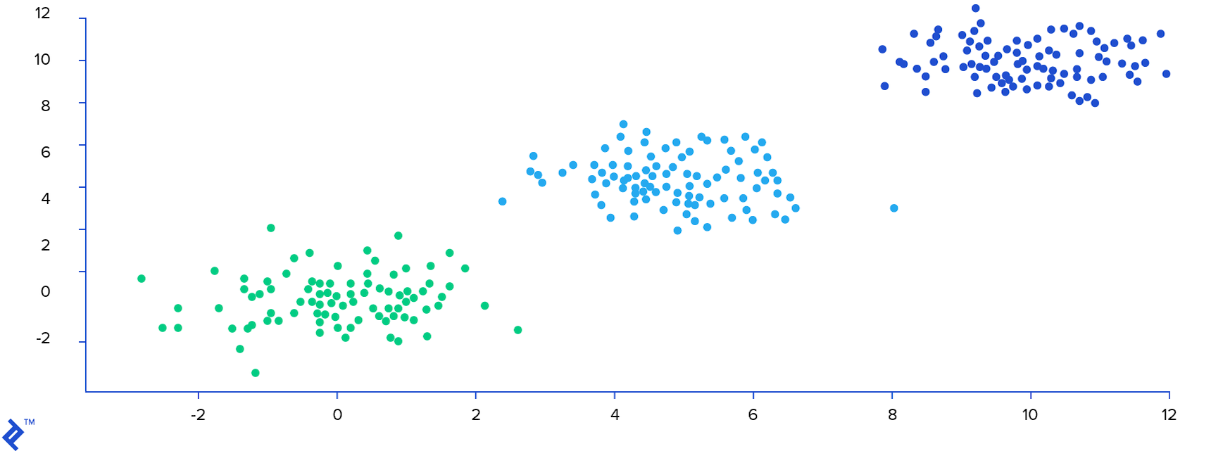
Unsupervised algorithms try to find structure in the data without explicitly being provided with labels. $k$-means is one of the examples of unsupervised algorithms which tries to find optimal clusters in the data. Below is an image with 300 data points. $k$-means algorithms found the structure in the data and assigned a cluster label to each data point. Each cluster has its own color.
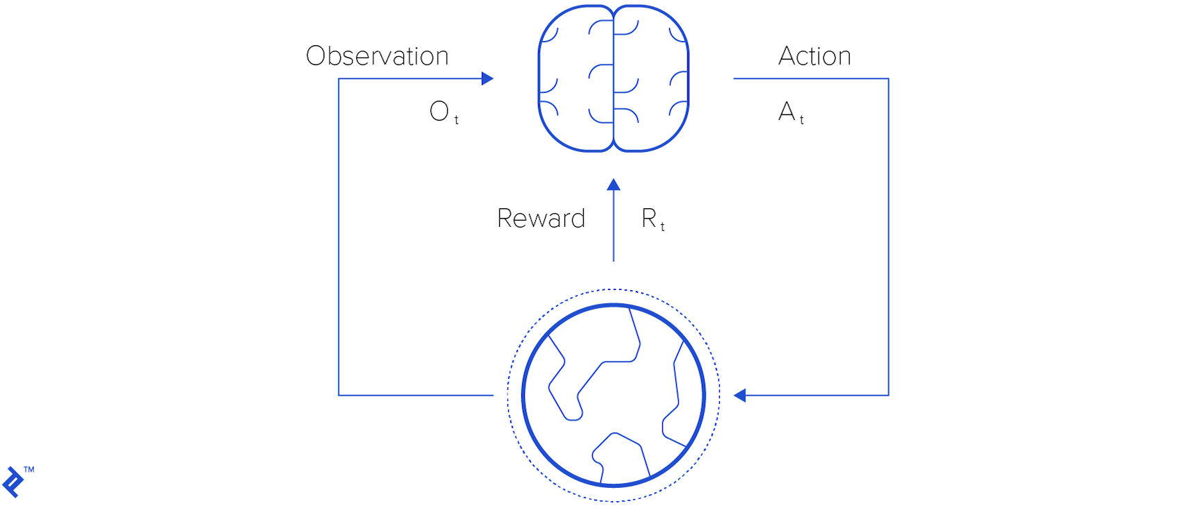
Reinforcement learning uses rewards: Sparse, time-delayed labels. An agent takes action, which changes the environment, from which it can get a new observation and reward. An observation is the stimulus an agent perceives from the environment. It can be what the agent sees, hears, smells, and so on.
A reward is given to the agent when it takes an action. It tells the agent how good the action is. By perceiving observations and rewards, an agent learns how to optimally behave in the environment. I’ll get into this in more detail below.
Active, Passive, and Inverse Reinforcement Learning
There are a few different approaches to this technique. First of all, there’s active reinforcement learning, which we’re using here. In contrast, there’s passive reinforcement learning, where rewards are merely another type of observation, and decisions are instead made according to a fixed policy.
Finally, inverse reinforcement learning tries to reconstruct a reward function given the history of actions and their rewards in various states.
Generalization, Overfitting, and Underfitting
Any fixed instance of parameters and hyperparameters is called a model. Machine learning experiments usually consist of two parts: Training and testing.
During the training process, learnable parameters are tuned using training data. In the test process, learnable parameters are frozen, and the task is to check how well the model makes predictions on previously unseen data. Generalization is the ability of a learning machine to perform accurately on a new, unseen example or task after having experienced a learning dataset.
If a model is too simple with respect to the data, it will not be able to fit the training data and it will perform poorly both on the training dataset and the test dataset. In that case, we say the model is underfitting.
If a machine learning model performs well on a training dataset, but poorly on a test dataset, we say that it’s overfitting. Overfitting is the situation where a model is too complex with respect to the data. It can perfectly fit training data, but it is adapted so much to the training dataset that it performs poorly on test data—i.e., it simply doesn’t generalize.
Below is an image showing underfitting and overfitting compared with a balanced situation between the overall data and the prediction function.

Scalability
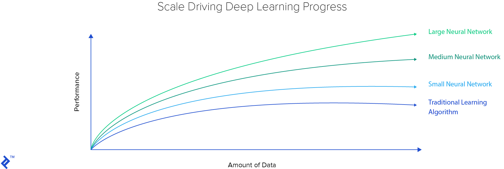
Data is crucial in building machine learning models. Usually, traditional learning algorithms don’t require too much data. But because of their limited capacity, performance is limited as well. Below is a plot showing how deep learning methods scale well compared to traditional machine learning algorithms.
Neural Networks
Neural networks consist of multiple layers. The image below shows a simple neural network with four layers. The first layer is the input layer, and the last layer is the output layer. The two layers between the input and output layers are hidden layers.
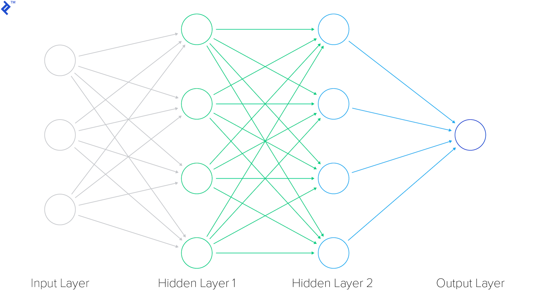
If a neural network has more than one hidden layer, we call it a deep neural network. The input set $ X $ is given to the neural network and the output $ y $ is obtained. Learning is done using a backpropagation algorithm which combines a loss function and an optimizer.
Backpropagation consists of two parts: a forward pass and a backward pass. In the forward pass, input data is put on the input of the neural network and output is obtained. The loss between the ground truth and the prediction is calculated, and then in the backward pass, neural networks’ parameters are tuned with respect to the loss.
Convolutional Neural Network
One neural network variation is the convolutional neural network. It’s primarily used for computer vision tasks.
The most important layer in convolutional neural networks is the convolutional layer (hence the name). Its parameters are made of learnable filters, also called kernels. Convolutional layers apply a convolution operation to the input, passing the result to the next layer. The convolution operation reduces the number of learnable parameters, functioning as a kind of heuristics and making the neural network easier to train.
Below is how one convolutional kernel in a convolutional layer works. The kernel is applied to the image and a convolved feature is obtained.

ReLU layers are used to introduce non-linearities in the neural network. Non-linearities are important because with them we can model all kind of functions, not only linear ones, making neural network a universal function approximator. This makes a ReLU function be defined like this:
\[ReLU = \max(0, x)\]ReLU is one of the examples of so-called activation functions used to introduce non-linearities in neural networks. Examples of other activation functions include sigmoid and hyper-tangent functions. ReLU is the most popular activation function because it is shown that it makes neural network train more efficiently compared to other activation functions.
Below is a plot of a ReLU function.
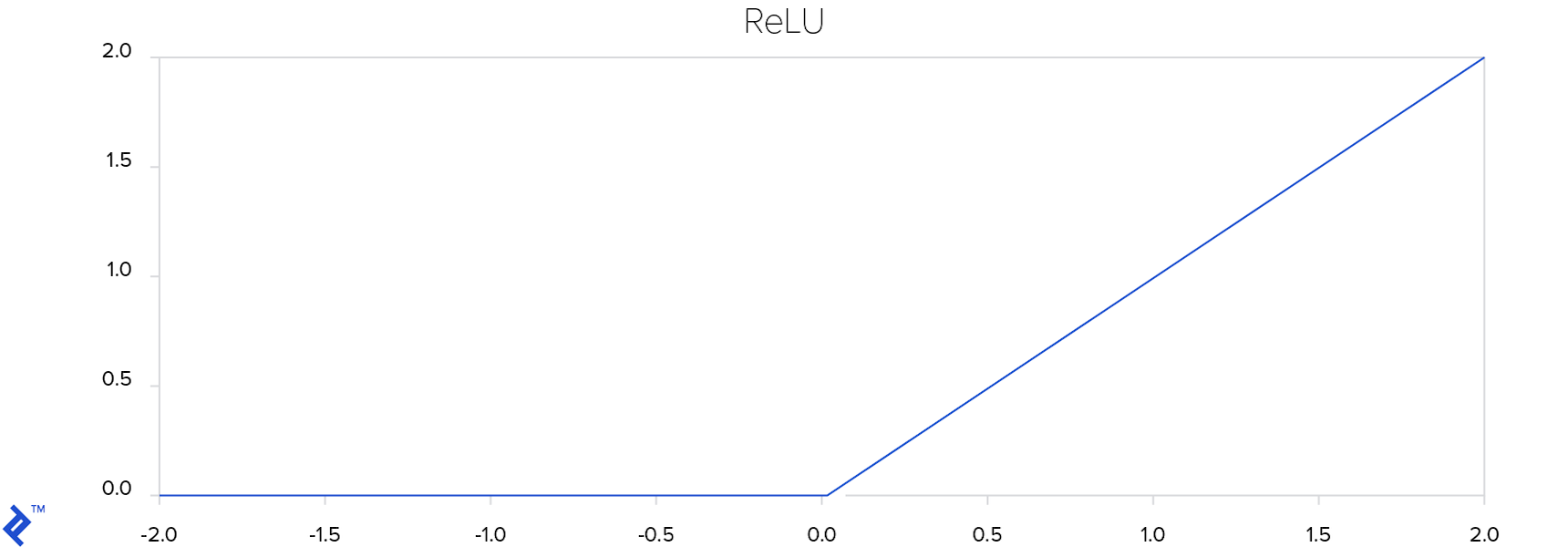
As you can see, this ReLU function simply changes negative values to zeros. This helps prevent the vanishing gradient problem. If a gradient vanishes, it will not have large impact in tuning the neural network’s weight.
A convolutional neural network consists of multiple layers: Convolutional layers, ReLU layers, and fully connected layers. Fully connected layers connect every neuron in one layer to every neuron in another layer, as seen with the two hidden layers in the image at the beginning of this section. The last fully connected layer maps outputs from the previous layer to, in this case, number_of_actions values.
Applications
Deep learning is successful and outperforms classical machine learning algorithms in several machine learning subfields, including computer vision, speech recognition, and reinforcement learning. These fields of deep learning are applied in various real-world domains: Finance, medicine, entertainment, etc.
Reinforcement Learning
Reinforcement learning is based around an agent. An agent takes actions in an environment and gets observations and rewards from it. An agent needs to be trained to maximize cumulative reward. As noted in the introduction, with classical machine learning algorithms, machine learning engineers need to do feature extraction, i.e., create good features which represent the environment well and which are fed into a machine learning algorithm.
Using deep learning, it’s possible to create an end-to-end system that takes high-dimensional input—e.g. video—and from it, it learns the optimal strategy for an agent to take good actions.
In 2013, London AI startup DeepMind created a great breakthrough in learning to control agents directly from high-dimensional sensory inputs. They published a paper, Playing Atari with Deep Reinforcement Learning, in which they showed how they taught an artificial neural network to play Atari games just from looking at the screen. They were acquired by Google, and then published a new paper in Nature with some improvements: Human-level control through deep reinforcement learning.
As opposed to other machine learning paradigms, reinforcement learning doesn’t have a supervisor, only a reward signal. Feedback is delayed: It is not instantaneous as in supervised learning algorithms. Data is sequential and an agent’s actions affect the subsequent data it receives.
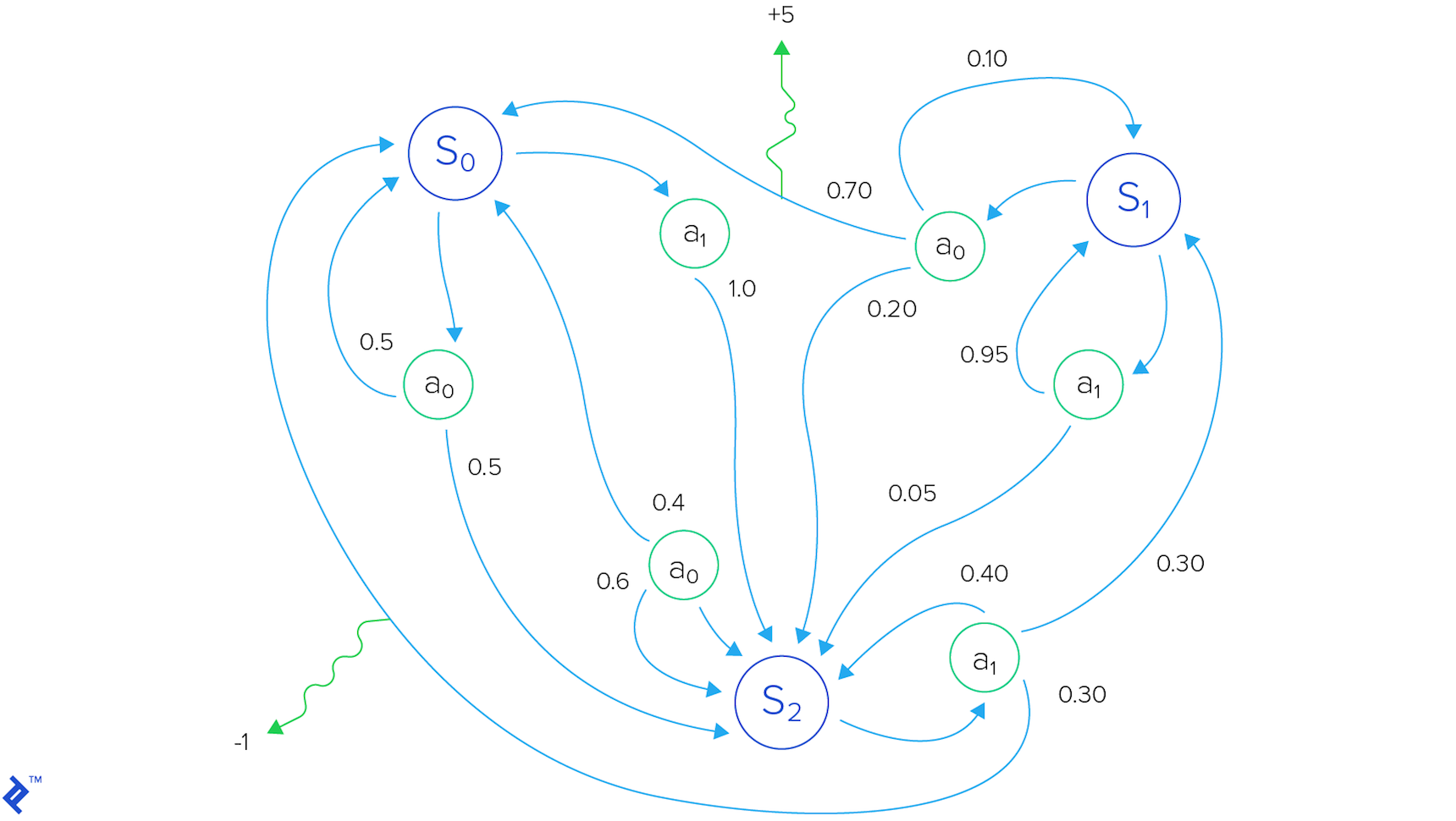
Now, an agent is situated in its environment, which is in a certain state. To describe this in more detail, we use a Markov decision process, which is a formal way of modeling this reinforcement learning environment. It’s made up of a set of states, a set of possible actions, and rules (e.g., probabilities) for transitioning from one state to another.
The agent is able to perform actions, transforming the environment. We call the reward $ R_t $. It’s a scalar feedback signal indicating how well the agent is doing at step $t$.
For good long-term performance, not only immediate rewards but also future rewards must be taken into account. The total reward for one episode from time step $t$ is $ R_t = r_t + r_{t+1} + r_{t+2} + \ldots + r_n $. The future is uncertain and the further we go in the future, the more future predictions may diverge. Because of that, a discounted future reward is used: $ R_t = r_t +\gamma r_{t+1} + \gamma^2r_{t+2} + \ldots + \gamma^{n-t}r_n = r_t + \gamma R_{t+1} $. An agent should choose the action which maximizes the discounted future reward.
Deep Q-learning
The $ Q(s, a) $ function represents the maximum discounted future reward when action $ a $ is performed
The estimation of a future reward is given by the Bellman equation: $ Q(s, a) = r + \gamma \max_{a’}Q(s’, a’) $ . In other words, the maximum future reward given a state $ s $ and an action $ a $ is the immediate reward plus maximum future reward for the next state.
The approximation of Q-values using non-linear functions (neural networks) is not very stable. Because of that, experience replay is used for stability. Experience during episodes in a training session are stored in a replay memory. Random mini-batches from the replay memory are used instead of using the most recent transition. This breaks the similarity of subsequent training samples which would otherwise drive the neural network into a local minimum.
There are two more important aspects to mention about deep Q-learning: Exploration and exploitation. With exploitation, the best decision given the current information is made. Exploration gathers more information.
When the algorithm performs an action proposed by the neural network, it is doing exploitation: It exploits the neural network’s learnt knowledge. In contrast, an algorithm can take a random action, exploring new possibilities and introducing potential new knowledge to the neural network.
The “Deep Q-learning algorithm with Experience Replay” from DeepMind’s paper Playing Atari with Deep Reinforcement Learning is shown below.
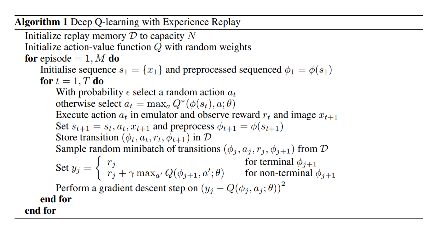
DeepMind refers to convolutional networks trained with their approach as Deep Q-networks (DQN).
Deep Q-learning Example Using Flappy Bird
Flappy Bird was a popular mobile game originally developed by Vietnamese video game artist and programmer Dong Nguyen. In it, the player controls a bird and tries to fly between green pipes without hitting them.
Below is a screenshot from a Flappy Bird clone coded using PyGame:
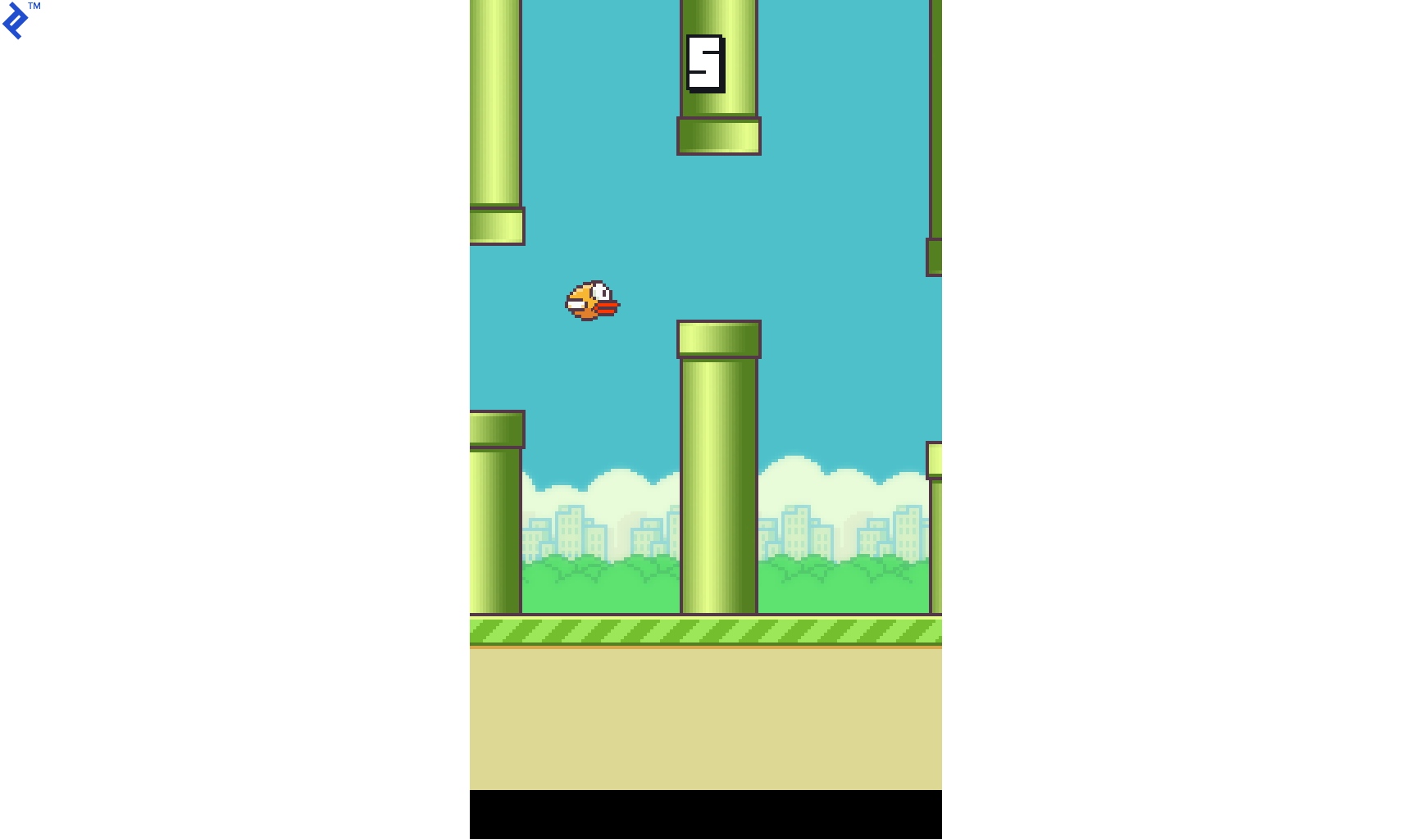
The clone has since been forked and modified: The background, sounds, and different bird and pipes styles have been removed and the code has been adjusted so it can easily be used with simple reinforcement learning frameworks. The modified game engine is taken from this TensorFlow project:
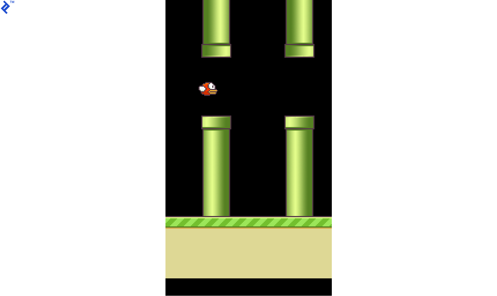
But instead of using TensorFlow, I’ve built a deep reinforcement learning framework using PyTorch. PyTorch is a deep learning framework for fast, flexible experimentation. It provides tensors and dynamic neural networks in Python with strong GPU acceleration.
The neural network architecture is the same as DeepMind used in the paper Human-level control through deep reinforcement learning.
| Layer | Input | Filter size | Stride | Number of filters | Activation | Output |
|---|---|---|---|---|---|---|
| conv1 | 84x84x4 | 8x8 | 4 | 32 | ReLU | 20x20x32 |
| conv2 | 20x20x32 | 4x4 | 2 | 64 | ReLU | 9x9x64 |
| conv3 | 9x9x64 | 3x3 | 1 | 64 | ReLU | 7x7x64 |
| fc4 | 7x7x64 | 512 | ReLU | 512 | ||
| fc5 | 512 | 2 | Linear | 2 |
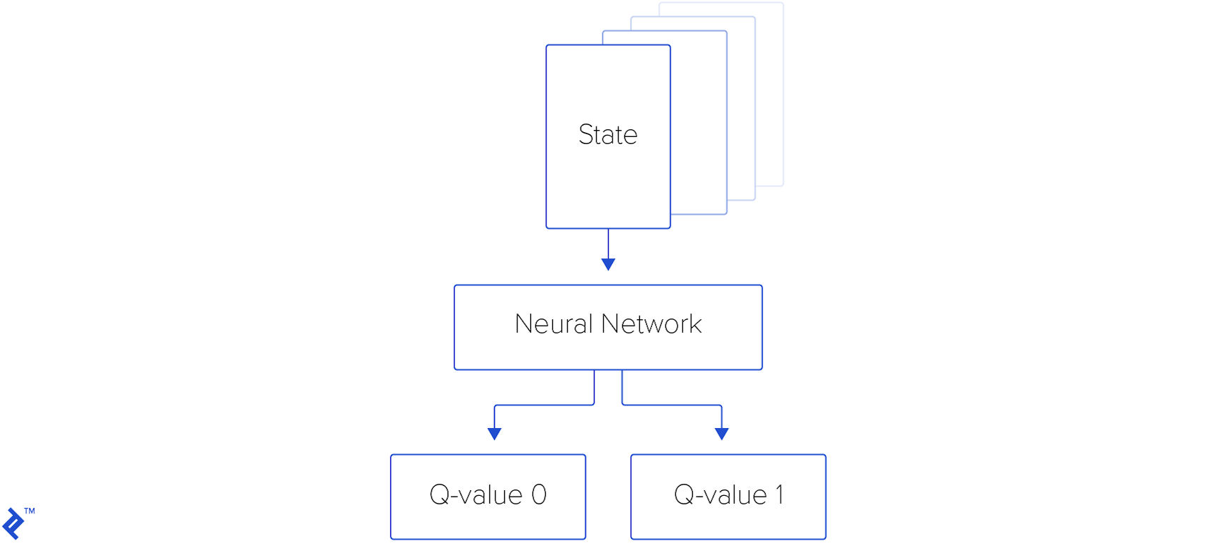
There are three convolutional layers and two fully connected layers. Each layer uses ReLU activation, except the last one, which uses linear activation. The neural network outputs two values representing the player’s only possible actions: “Fly up” and “do nothing.”
The input consists of four consecutive 84x84 black-and-white images. Below is an example of four images which are fed to the neural network.
You’ll notice that the images are rotated. That is because the output of the clone’s game engine is rotated. But if the neural network is taught and then tested using such images, it will not affect its performance.

You may also notice that the image is cropped so that the floor is omitted, because it is irrelevant for this task. All pixels that represent pipes and the bird are white and all pixels that represent the background are black.
This is part of the code that defines the neural network. Neural networks’ weights are initialized to follow the uniform distribution $\mathcal{U}(-0.01, 0.01)$. The bias part of neural networks’ parameters is set to 0.01. Several different initializations were tried (Xavier uniform, Xavier normal, Kaiming uniform, Kaiming normal, uniform, and normal), but the above initialization made the neural network converge and train the fastest. The size of the neural network is 6.8 MB.
class NeuralNetwork(nn.Module):

    def __init__(self):
        super(NeuralNetwork, self).__init__()

        self.number_of_actions = 2
        self.gamma = 0.99
        self.final_epsilon = 0.0001
        self.initial_epsilon = 0.1
        self.number_of_iterations = 2000000
        self.replay_memory_size = 10000
        self.minibatch_size = 32

        self.conv1 = nn.Conv2d(4, 32, 8, 4)
        self.relu1 = nn.ReLU(inplace=True)
        self.conv2 = nn.Conv2d(32, 64, 4, 2)
        self.relu2 = nn.ReLU(inplace=True)
        self.conv3 = nn.Conv2d(64, 64, 3, 1)
        self.relu3 = nn.ReLU(inplace=True)
        self.fc4 = nn.Linear(3136, 512)
        self.relu4 = nn.ReLU(inplace=True)
        self.fc5 = nn.Linear(512, self.number_of_actions)

    def forward(self, x):
        out = self.conv1(x)
        out = self.relu1(out)
        out = self.conv2(out)
        out = self.relu2(out)
        out = self.conv3(out)
        out = self.relu3(out)
        out = out.view(out.size()[0], -1)
        out = self.fc4(out)
        out = self.relu4(out)
        out = self.fc5(out)

        return out
In the constructor, you’ll notice that there are hyperparameters defined. Hyperparameter optimization is not done for the purpose of this blog post. Instead, hyperparameters are mostly used from DeepMind’s papers. Here, some of the hyperparameters are scaled to be lower than in DeepMind’s paper, because Flappy Bird is less complex than the Atari games they used for tuning.
Also, epsilon is changed to be much more reasonable for this game. DeepMind uses an epsilon of one, but here we use 0.1. This is because higher epsilons force the bird to flap a lot, which pushes the bird toward the upper border of the screen, always eventually resulting in the bird crashing into a pipe.
The reinforcement learning code has two modes: Train and test. During the test phase, we can see how well the reinforcement learning algorithm has learned to play the game. But first, the neural network needs to be trained. We need to define the loss function to be minimized and the optimizers which will minimize the loss function. We’ll use the Adam optimization method and the mean squared error for the loss function:
optimizer = optim.Adam(model.parameters(), lr=1e-6)
criterion = nn.MSELoss()
The game should be instantiated:
game_state = GameState()
Replay memory is defined as a Python list:
replay_memory = []
Now we need to initialize the first state. An action is two-dimensional tensor:
- [1, 0] represents “do nothing”
- [0, 1] represents “fly up”
The frame_step method gives us next screen, reward, and information as to whether the next state is terminal. The reward is 0.1 for each bird’s move without dying when it is not passing through a pipe, 1 if the bird successfully pass through a pipe and -1 if the bird crashes.
The resize_and_bgr2gray function crops the floor, resizes screen to an 84x84 image, and changes the color space from BGR to black-and-white. The image_to_tensor function converts the image to a PyTorch tensor and puts it in GPU memory if CUDA is available. Finally, the last four sequential screens are concatenated together and are ready to be sent to the neural network.
action = torch.zeros([model.number_of_actions], dtype=torch.float32)
action[0] = 1
image_data, reward, terminal = game_state.frame_step(action)
image_data = resize_and_bgr2gray(image_data)
image_data = image_to_tensor(image_data)
state = torch.cat((image_data, image_data, image_data, image_data)).unsqueeze(0)
The initial epsilon is set using this line of code:
epsilon = model.initial_epsilon
The main infinite loop follows. Comments are written in the code and you can compare code with the Deep Q-learning with Experience Replay algorithm written above.
The algorithm samples mini-batches from replay memory and updates the neural network’s parameters. Actions are executed using epsilon greedy exploration. Epsilon is being annealed over time. The loss function being minimized is $ L = \frac{1}{2}\left[\max_{a’}Q(s’, a’) - Q(s, a)\right]^2 $ . $ Q(s, a) $ is the ground truth value calculated using the Bellman equation and $ \max_{a’}Q(s’, a’) $ is obtained from the neural network. The neural network gives two Q-values for the two possible actions and the algorithm takes the action with the highest Q-value.
while iteration < model.number_of_iterations:
    # get output from the neural network
    output = model(state)[0]

    # initialize action
    action = torch.zeros([model.number_of_actions], dtype=torch.float32)
    if torch.cuda.is_available():  # put on GPU if CUDA is available
        action = action.cuda()

    # epsilon greedy exploration
    random_action = random.random() <= epsilon
    if random_action:
        print("Performed random action!")
    action_index = [torch.randint(model.number_of_actions, torch.Size([]), dtype=torch.int)
                    if random_action
                    else torch.argmax(output)][0]

    if torch.cuda.is_available():  # put on GPU if CUDA is available
        action_index = action_index.cuda()

    action[action_index] = 1

    # get next state and reward
    image_data_1, reward, terminal = game_state.frame_step(action)
    image_data_1 = resize_and_bgr2gray(image_data_1)
    image_data_1 = image_to_tensor(image_data_1)
    state_1 = torch.cat((state.squeeze(0)[1:, :, :], image_data_1)).unsqueeze(0)

    action = action.unsqueeze(0)
    reward = torch.from_numpy(np.array([reward], dtype=np.float32)).unsqueeze(0)

    # save transition to replay memory
    replay_memory.append((state, action, reward, state_1, terminal))

    # if replay memory is full, remove the oldest transition
    if len(replay_memory) > model.replay_memory_size:
        replay_memory.pop(0)

    # epsilon annealing
    epsilon = epsilon_decrements[iteration]

    # sample random minibatch
    minibatch = random.sample(replay_memory, min(len(replay_memory), model.minibatch_size))

    # unpack minibatch
    state_batch = torch.cat(tuple(d[0] for d in minibatch))
    action_batch = torch.cat(tuple(d[1] for d in minibatch))
    reward_batch = torch.cat(tuple(d[2] for d in minibatch))
    state_1_batch = torch.cat(tuple(d[3] for d in minibatch))

    if torch.cuda.is_available():  # put on GPU if CUDA is available
        state_batch = state_batch.cuda()
        action_batch = action_batch.cuda()
        reward_batch = reward_batch.cuda()
        state_1_batch = state_1_batch.cuda()

    # get output for the next state
    output_1_batch = model(state_1_batch)

    # set y_j to r_j for terminal state, otherwise to r_j + gamma*max(Q)
    y_batch = torch.cat(tuple(reward_batch[i] if minibatch[i][4]
                              else reward_batch[i] + model.gamma * torch.max(output_1_batch[i])
                              for i in range(len(minibatch))))

    # extract Q-value
    q_value = torch.sum(model(state_batch) * action_batch, dim=1)

    # PyTorch accumulates gradients by default, so they need to be reset in each pass
    optimizer.zero_grad()

    # returns a new Tensor, detached from the current graph, the result will never require gradient
    y_batch = y_batch.detach()

    # calculate loss
    loss = criterion(q_value, y_batch)

    # do backward pass
    loss.backward()
    optimizer.step()

    # set state to be state_1
    state = state_1
Now that all the pieces are in place, here’s a high-level overview of the data flow using our neural network:
Here is one short sequence with a trained neural network.
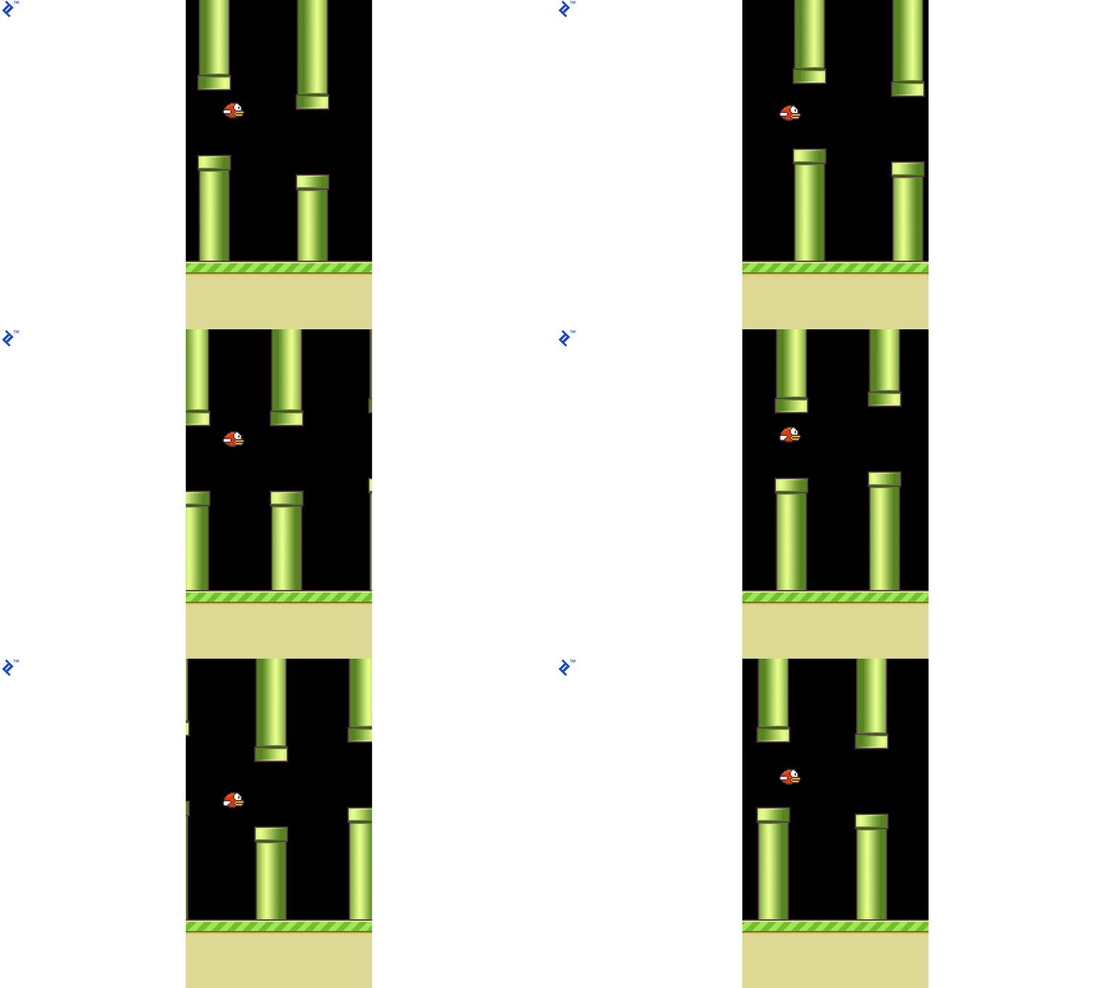
The neural network shown above was trained using a high-end Nvidia GTX 1080 GPU for a few hours; using a CPU-based solution instead, this particular task would take several days. The game engine’s FPS were set to a very large number during training: 999…999—in other words, as many frames per second as possible. In testing phase, the FPS was set to 30.
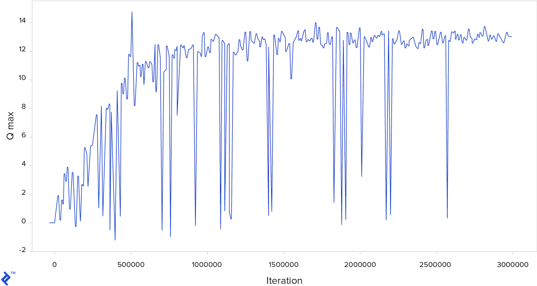
Below is a chart showing how the maximum Q-value changed during iterations. Every 10,000th iteration is shown. A downward spike means that for a particular frame (one iteration being one frame) the neural network predicts the bird will get a very low reward in the future—i.e., it will crash very soon.
The full code and pretrained model are available here.
Deep Reinforcement Learning: 2D, 3D, and Even Real Life
In this PyTorch reinforcement learning tutorial, I showed how a computer can learn to play Flappy Bird without any previous knowledge about the game, using only a trial-and-error approach as a human would do when encountering the game for the first time.
It is interesting that the algorithm can be implemented in a few lines of code using the PyTorch framework. The paper on which the method in this blog is based is relatively old, and a lot of newer papers with various modifications which enable faster convergence are available. Since then, deep reinforcement learning has been used for playing 3D games and in real-world robotic systems.
Companies like DeepMind, Maluuba, and Vicarious are working intensively on deep reinforcement learning. Such technology was used in AlphaGo, which beat Lee Sedol, one of the world’s best players at Go. At the time, it was considered that it would take at least ten years until machines could defeat the best players at Go.
The flood of interest and investments in deep reinforcement learning (and in artificial intelligence in general) might even lead to potential artificial general intelligence (AGI)—human-level intelligence (or even beyond) that can be expressed in the form of an algorithm and simulated on computers. But AGI will have to be the subject of another article.
References:
Further Reading on the Toptal Blog:
Understanding the basics
What is unsupervised learning?
Unsupervised learning is an approach to machine learning that finds structure in data. Unlike with supervised learning, data is not labeled.
What is passive reinforcement learning?
In passive reinforcement learning, the agent learns and follows a policy. It gets “rewards,” but can only observe them, whether they are good or not. In contrast, active reinforcement learning has agents learn to take the best action for each state to maximize cumulative future rewards.
What is inverse reinforcement learning?
In reinforcement learning, an agent has access to feedback in the form of a “reward” every time it takes some action in some state in the environment. Inverse reinforcement learning tries to reconstruct a reward function given the history of rewards received for actions in certain states.
What are the types of neural networks?
Many neural networks types are based on the combinations of layers they use, e.g. convolutional layers, fully connected layers, and LSTM layers. Types of neural networks include convolutional neural networks (CNNs), recurrent neural networks (RNNs), and multilayer perceptron (MLP or “vanilla”) neural networks.
What is DeepMind AI?
DeepMind Technologies Limited is a London-based artificial intelligence company. They developed AlphaGo, which beat Lee Sedol, a world champion in Go. The company was acquired by Google in 2014.
Zagreb, Croatia
Member since September 27, 2017
About the author
Co-founder of Poze and CEO of an AI R&D/consulting company, Neven has an MCS degree and has built a face-recognition system in TensorFlow.
