Sound Logic and Monotonic AI Models

AI is fast becoming an amazing asset, having achieved superhuman levels of performance in domains such as image recognition, Go, and even poker. Many are excited about the future of AI and humanity. At the same time, there is a general sense that AI does suffer from one pesky flaw: AI in its current state can be unpredictably unreliable.

The classical example is the Jeopardy! IBM Challenge, during which Watson, the IBM AI, cleaned the board with ease, only to miss the “Final Jeopardy!” question, which was under the category of US Cities: “Its largest airport is named for a World War II hero; its second largest for a World War II battle.” Watson answered, “What is Toronto?????”—the extra question marks (and low wager) indicating its doubt.

So even though AI has the capacity for fairy-tale-like performance for large periods of time—months, years, decades even—there is always this nagging possibility that all of a sudden, it will mysteriously blunder.

Most concerning to us humans is not that the AI will make a mistake, but how “illogical” the mistake will be. In Watson’s case, someone who doesn’t know the answer to the question would “logically” try to at least guess a major US city. I believe that this is one of the main reasons we don’t yet have public adoption of self-driving cars: Even if self-driving cars may be statistically safer, we fear that their underlying AI might unexpectedly blunder in a similar sense to Watson, but with much more serious repercussions.

This got me wondering, could the right AI model fix this issue? Could the right AI have the capability to make sound decisions in critical moments, even when it doesn’t have all the answers? Such AI would be able to change the course of technology and enable us the fairy-tale-like benefits of AI…

I believe the answer to these questions is yes. I believe that mistakes like Watson’s may be avoidable with the use of improved, more logically constrained models, the early prototype of which are called monotonic machine learning models. Without going into details just yet, with the proper monotonic AI model:

• A self-driving car would be safer, as the detection of even the smallest amount of human signal would always suffice to activate a safety protocol even in the presence of a large amount of other signal.
• Machine learning (ML) systems would be more robust to adversarial attacks and unexpected situations.
• ML performance would be more logical and humanly understandable.

I believe we are moving from an era of great growth in the computational and algorithmic power of AI to an era of finesse, effectiveness, and understanding in AI, and monotonic machine learning models are the first step in this exciting journey. Monotonic models make AI more “logical.”

Editor’s note: Readers looking to take their own first step in understanding ML basics are encouraged to read our introductory article on ML.

The Theory of Monotonic AI Models

So what is a monotonic model? Loosely speaking, a monotonic model is an ML model that has some set of features (monotonic features) whose increase always leads the model to increase its output.

In real life, many pairs of variables exhibit monotonic relationships. For example:

• The gas price for a trip is monotonically increasing in the distance driven.
• The likelihood of receiving a loan is greater with better credit.
• The expected driving time increases with the amount of traffic.
• Revenue increases with the click rate on an ad.

Though these logical relationships are clear enough, for an ML model that is interpolating using limited data and no domain knowledge, they might not be. In fact, the model might interpolate them incorrectly, resulting in ridiculous and wacky predictions. Machine learning models that do capture such knowledge perform better in practice (by avoiding overfitting), are easier to debug, and are more interpretable. In most use cases, the monotonic model should be used in conjunction with an ordinary model, as part of an ensemble of learners.

One place where monotonic AI models really shine is in adversarial robustness. Monotonic models are “hardened” machine learning models, meaning they are resistant to adversarial attacks. Attackers who are able to manipulate only non-monotonic features are unable to evade the monotonic AI model because they are unable to alter the label of the example with respect to the monotonic AI model.

Use Cases for Monotonic AI Models

So far, this discussion has been entirely theoretical. Let’s discuss some real-life use cases.

Use Case #1: Malware Detection

One of the coolest use cases for monotonic AI models has to be their use in malware detection. Implemented as part of Windows Defender, a monotonic model is present in every up-to-date Windows device, quietly protecting users from malware.

In one scenario, malware authors impersonated legitimate, registered businesses to defraud certificate authorities, successfully digitally code-signing their malware with trusted certificates. A naive malware classifier is likely to use code-signing as a feature and would indicate such samples to be benign.

But not so in the case of Windows Defender’s monotonic AI model, whose monotonic features are only the features that indicate malware. No matter how much “benign” content malware authors inject into their malware, Windows Defender’s monotonic AI model would continue to catch the sample and defend users from damage.

In my course, Machine Learning for Red Team Hackers, I teach several techniques for evading ML-based malware classifiers. One of the techniques consists of stuffing a malicious sample with “benign” content/features to evade naive ML models. Monotonic models are resistant to this attack and force malicious actors to work much harder if they are to have any hope of evading the classifier.

Use Case #2: Content Filtering

Suppose a team is constructing a web-surfing content filter for school libraries. A monotonic AI model is a great candidate to use here because a forum that contains inappropriate content might also contain plenty of acceptable content.

A naive classifier might weigh the presence of “appropriate” features against the presence of “inappropriate” features. But that won’t do since we don’t want our children accessing inappropriate content, even if it makes up only a small fraction of the content.

Use Case #3: Self-driving Car AI

Imagine constructing a self-driving car algorithm. It looks at an image and sees a green light. It also sees a pedestrian. Should it weigh the signal of each against one another? Absolutely not. The presence of a pedestrian is sufficient to make a decision to stop the car. The presence of pedestrians should be viewed as a monotonic feature, and a monotonic AI model should be used in this scenario.

Use Case #4: Recommendation Engines

Recommendation engines are a great use case for monotonic AI models. In general, they might have many inputs about each product: star rating, price, number of reviews, etc. With all other inputs being equal, such as star ratings and price, we would prefer the product that has a greater number of reviews. We can enforce such logic using a monotonic AI model.

Use Case #5: Spam and Phishing Filtering

This use case is similar to the malware detection use case. Malicious users may inject their spam or phishing emails with benign-seeming terms to fool spam filters. A monotonic AI model will be immune to that.

Implementation and Demonstration

When it comes to freely available implementations of monotonic AI models, three stand out as best-supported: XGBoost, LightGBM, and TensorFlow Lattice.

Monotonic ML XGBoost Tutorial

XGBoost is considered one of the best-performing algorithms on structured data, based on years of empirical research and competition. In addition, monotonicity has been implemented in XGBoost.

The following demonstration XGBoost tutorial on how to use monotonic ML models has an accompanying Python repo.

Start by importing a few libraries:

import random
import numpy as np
import matplotlib.pyplot as plt
%matplotlib inline
from sklearn.metrics import confusion_matrix
import seaborn as sns

sns.set(font_scale=1.4)

The scenario we are going to model is a content filtering or malware database. We will have some benign_features, which model, e.g., the amount of content related to “science,” “history,” and “sports,” or in the malware case, “code-signing” and “recognized authors.”

Also, we will have malicious_features, which model, e.g., the amount of content related to “violence” and “drugs,” or in the malware case, “the number of times calls to crypto libraries are made” and “a numerical measure of similarity to a known malware family.”

We will model the situation via a generative model. We generate a large number of data points at random, about half benign and half malicious, using the function:

def flip():
    """Simulates a coin flip."""
    return 1 if random.random() < 0.5 else 0

Each data point will randomly generate its features. A “benign” data point will have a higher bias for the benign features, while a “malicious” data point will have a higher bias for the malicious features.

We will use a triangular distribution, like so:

bins = [0.1 * i for i in range(12)]

plt.hist([random.triangular(0, 1, 1) for i in range(50000)], bins)

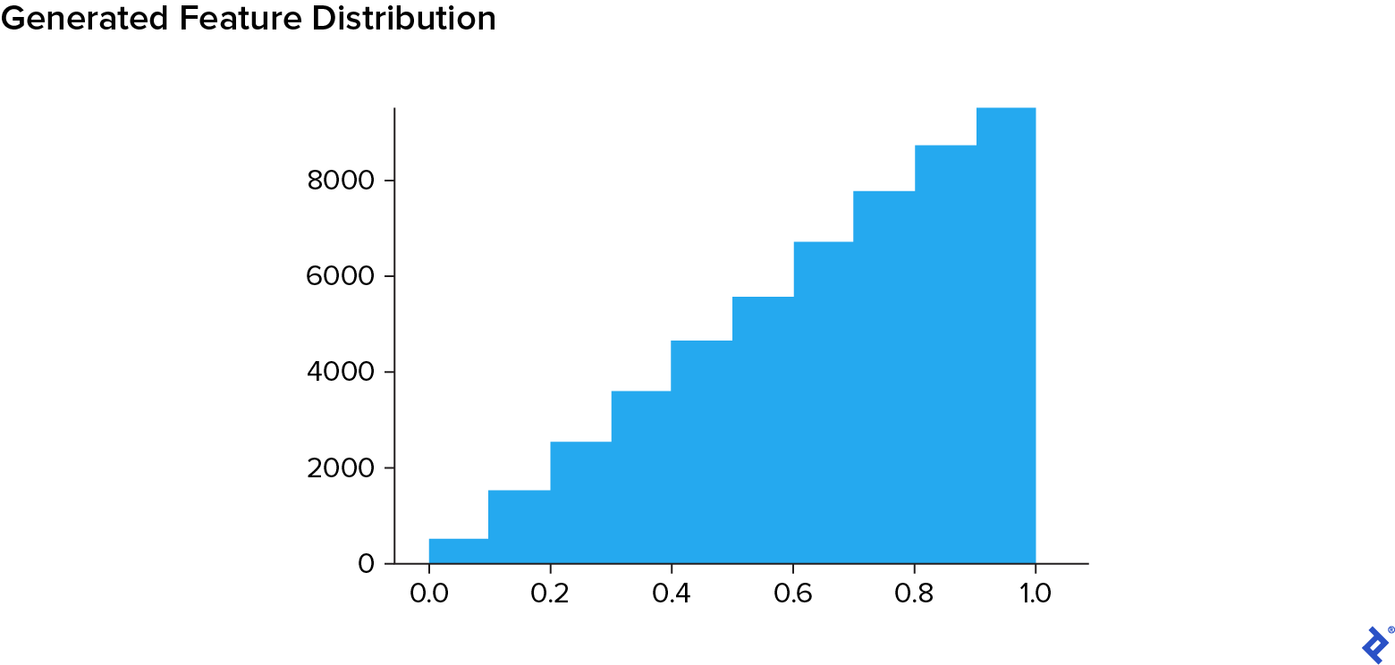
We’ll use this function to capture the above logic:

def generate():
    """Samples from the triangular distribution."""
    return random.triangular(0, 1, 1)

Then, we’ll proceed to create our dataset:

m = 100000
benign_features = 5
malicious_features = 5
n = benign_features + malicious_features
benign = 0
malicious = 1
X = np.zeros((m, n))
y = np.zeros((m))
for i in range(m):
    vec = np.zeros((n))
y[i] = flip()
if y[i] == benign:
    for j in range(benign_features):
        vec[j] = generate()
    for j in range(malicious_features):
        vec[j + benign_features] = 1 - generate()
else:
    for j in range(benign_features):
        vec[j] = 1 - generate()
    for j in range(malicious_features):
        vec[j + benign_features] = generate()
X[i, :] = vec

X contains the vectors of randomly generated features, while y contains the labels. This classification problem is not trivial.

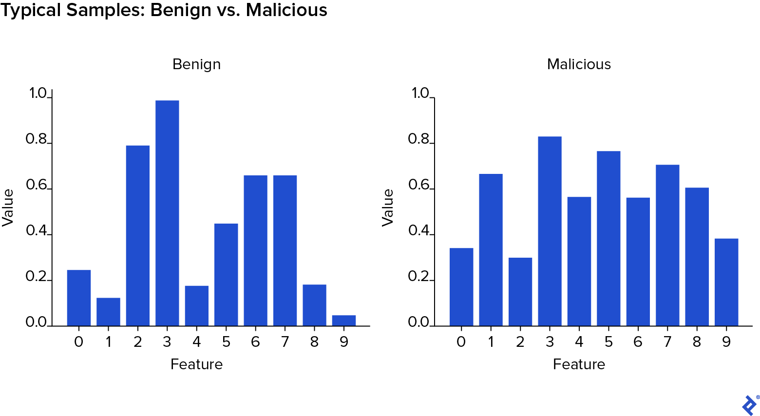
You can see that benign samples generally have greater weight in the first few features, whereas malicious samples generally have greater weight in the last few features.

With the data ready, let’s perform a simple training-testing split:

from sklearn.model_selection import train_test_split

X_train, X_test, y_train, y_test = train_test_split(X, y, test_size=0.2)

We’ll use a function to prep the data for use with our XGBoost tutorial:

import xgboost as xgb

def prepare_for_XGBoost(X, y):
    """Converts a numpy X and y dataset into a DMatrix for XGBoost."""
    return xgb.DMatrix(X, label=y)

dtrain = prepare_for_XGBoost(X_train, y_train)
dtest = prepare_for_XGBoost(X_test, y_test)
dall = prepare_for_XGBoost(X, y)

Now, let’s train and test a simple (non-monotonic) XGBoost model on the data. We will then print out the confusion matrix to see a numerical breakdown of the correctly labeled positive examples, correctly labeled negative examples, incorrectly labeled positive examples, and incorrectly labeled negative examples.

params = {"n_jobs": -1, "tree_method": "hist"}
model_no_constraints = xgb.train(params=params, dtrain=dtrain)
CM = predict_with_XGBoost_and_return_confusion_matrix(
    model_no_constraints, dtrain, y_train
)
plt.figure(figsize=(12, 10))
sns.heatmap(CM / np.sum(CM), annot=True, fmt=".2%", cmap="Blues")
plt.ylabel("True Label")
plt.xlabel("Predicted Label")
plt.title("Unconstrained model's training confusion matrix")
plt.show()
print()
CM = predict_with_XGBoost_and_return_confusion_matrix(
    model_no_constraints, dtest, y_test
)
plt.figure(figsize=(12, 10))
sns.heatmap(CM / np.sum(CM), annot=True, fmt=".2%", cmap="Blues")
plt.ylabel("True Label")
plt.xlabel("Predicted Label")
plt.title("Unconstrained model's testing confusion matrix")
plt.show()
model_no_constraints = xgb.train(params=params, dtrain=dall)

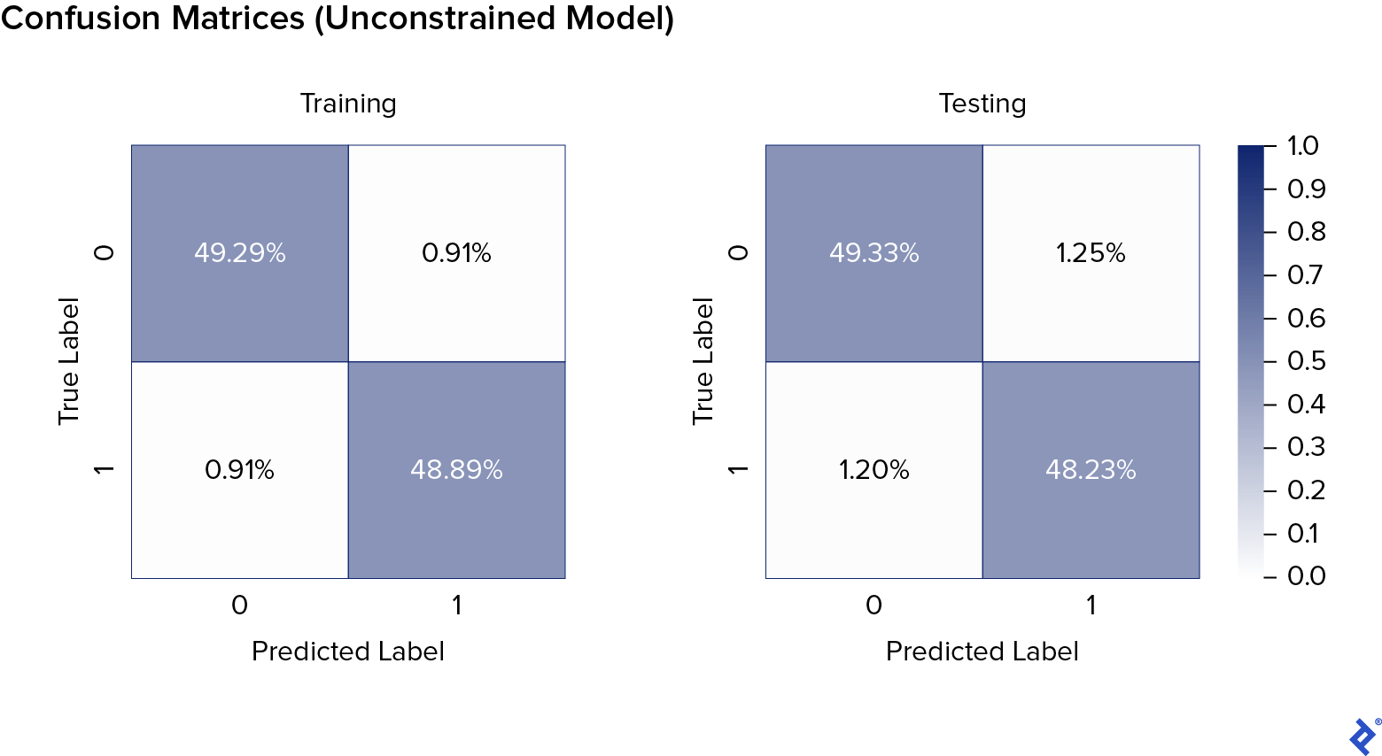
Looking at the results, we can see that there is no significant overfitting. We will compare these results to those of the monotonic models.

To that end, let’s train and test a monotonic XGBoost model. The syntax in which we pass in the monotone constraints is a sequence (f₀, f₁, …, f_N), where each f_i is one of -1, 0 or 1, depending on whether we want feature i to be monotonically decreasing, unconstrained, or monotonically increasing, respectively. In the case at hand, we specify the malicious features to be monotonic increasing.

params_constrained = params.copy()
monotone_constraints = (
    "("
    + ",".join([str(0) for m in range(benign_features)])
    + ","
    + ",".join([str(1) for m in range(malicious_features)])
    + ")"
)
print("Monotone constraints enforced are:")
print(monotone_constraints)
params_constrained["monotone_constraints"] = monotone_constraints
model_monotonic = xgb.train(params=params_constrained, dtrain=dtrain)
CM = predict_with_XGBoost_and_return_confusion_matrix(model_monotonic, dtrain, y_train)
plt.figure(figsize=(12, 10))
sns.heatmap(CM / np.sum(CM), annot=True, fmt=".2%", cmap="Blues")
plt.ylabel("True Label")
plt.xlabel("Predicted Label")
plt.title("Monotonic model's training confusion matrix")
plt.show()
print()
CM = predict_with_XGBoost_and_return_confusion_matrix(model_monotonic, dtest, y_test)
plt.figure(figsize=(12, 10))
sns.heatmap(CM / np.sum(CM), annot=True, fmt=".2%", cmap="Blues")
plt.ylabel("True Label")
plt.xlabel("Predicted Label")
plt.title("Monotonic model's testing confusion matrix")
plt.show()
model_monotonic = xgb.train(params=params_constrained, dtrain=dall)

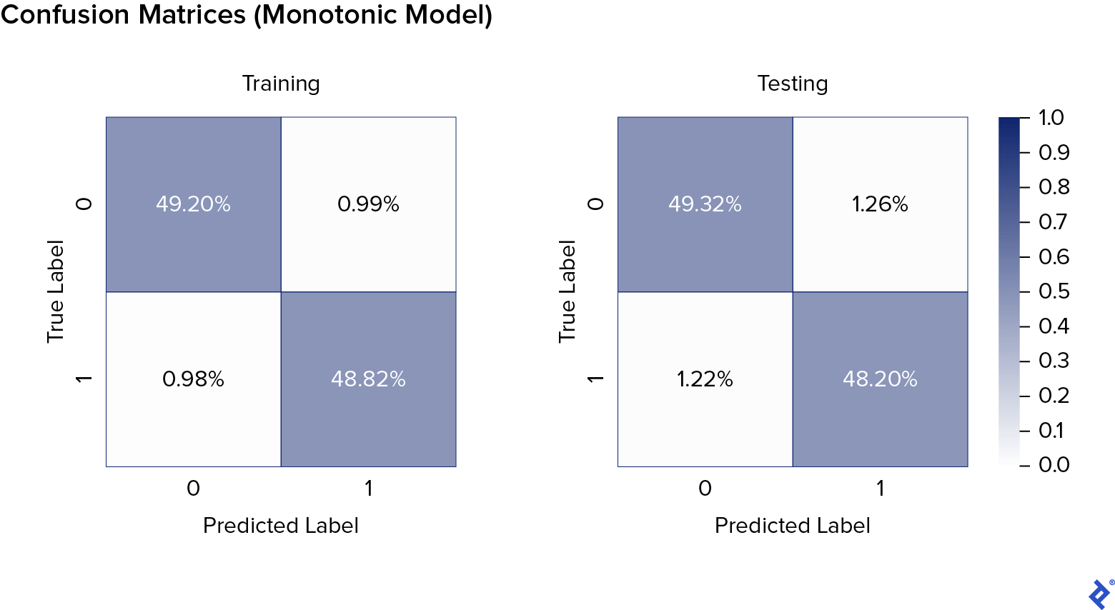
It’s clear that the performance of the monotonic model is the same as that of the unconstrained model.

Now, we are going to create an adversarial dataset. We are going to take all of the malicious samples and “stuff” their benign features by setting them all to 1. We will then see how the two models perform side by side.

X_adversarial = X[y == malicious]
y_adversarial = len(X_adversarial) * [malicious]
for i in range(len(X_adversarial)):
    vec = X_adversarial[i, :]
    for j in range(benign_features):
        vec[j] = 1
    X_adversarial[i, :] = vec

Let’s convert these to a form to be ingested by XGBoost:

dadv = prepare_for_XGBoost(X_adversarial, y_adversarial)

For the final step of our XGBoost tutorial, we’ll test the two machine learning model types:

CM = predict_with_XGBoost_and_return_confusion_matrix(
    model_no_constraints, dadv, y_adversarial
)
plt.figure(figsize=(12, 10))
sns.heatmap(CM / np.sum(CM), annot=True, fmt=".2%", cmap="Blues")
plt.ylabel("True Label")
plt.xlabel("Predicted Label")
plt.title("Unconstrained model's confusion matrix on adversarial dataset")
plt.show()

CM = predict_with_XGBoost_and_return_confusion_matrix(
    model_monotonic, dadv, y_adversarial
)
plt.figure(figsize=(12, 10))
sns.heatmap(CM / np.sum(CM), annot=True, fmt=".2%", cmap="Blues")
plt.ylabel("True Label")
plt.xlabel("Predicted Label")
plt.title("Monotonic model's confusion matrix on adversarial dataset")
plt.show()

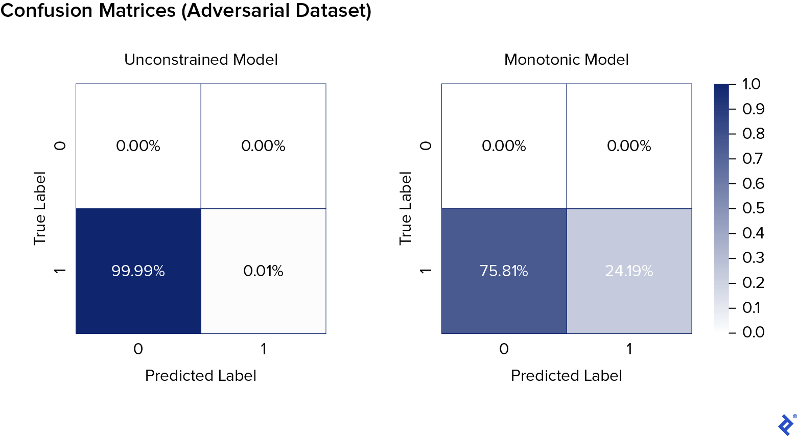
As you can see, the monotonic AI model was about 2,500 times more robust to adversarial attacks.

LightGBM

The syntax for using monotonic features in LightGBM is similar.

TensorFlow Lattice

TensorFlow Lattice is another framework for tackling monotonicity constraints and is a set of prebuilt TensorFlow Estimators as well as TensorFlow operators to build your own lattice models. Lattices are multi-dimensional interpolated look-up tables, meaning they are points evenly distributed in space (like a grid), along with function values at these points. According to the Google AI Blog:

“…the look-up table values are trained to minimize the loss on the training examples, but in addition, adjacent values in the look-up table are constrained to increase along given directions of the input space, which makes the model outputs increase in those directions. Importantly, because they interpolate between the look-up table values, the lattice models are smooth and the predictions are bounded, which helps to avoid spurious large or small predictions in the testing time.”

Tutorials for how to use TensorFlow Lattice can be found here.

Monotonic AI Models and the Future

From defending devices from malicious attacks to offering logical and helpful restaurant recommendations, monotonic AI models have proven to be a great boon to society and a wonderful tool to master. Monotonic models are here to usher us into a new era of safety, finesse, and understanding in AI. And so I say, here’s to monotonic AI models, here’s to progress.