Adversarial Machine Learning: How to Attack and Defend ML Models
The increasing accuracy of machine learning systems has resulted in a flood of applications using them. As machine learning models matured and improved, so did ways of attacking them.
In this article, Toptal Python Developer Pau Labarta Bajo examines the world of adversarial machine learning, explains how ML models can be attacked, and what you can do to safeguard them against attack.
Pau has extensive experience in quantitative finance. He combines love of statistics and machine learning with excellent Python skills.
Expertise
PREVIOUSLY AT

Nowadays, machine learning models in computer vision are used in many real-world applications, like self-driving cars, face recognition, cancer diagnosis, or even in next-generation shops in order to track which products customers take off the shelf so their credit card can be charged when leaving.
The increasing accuracy of these machine learning systems is quite impressive, so it naturally led to a veritable flood of applications using them. Although the mathematical foundations behind them were already studied a few decades ago, the relatively recent advent of powerful GPUs gave researchers the computing power necessary to experiment and build complex machine learning systems. Today, state-of-the art models for computer vision are based on deep neural networks with up to several million parameters, and they rely on hardware that was not available just a decade ago.
In 2012, Alex Krizhevsky et altri became the first to show how to implement a deep convolutional network, which at the time became the state-of-the art model in object classification. Since then, many improvements to their original model have been published, each of them giving an uplift in accuracy (VGG, ResNet, Inception, etc). As of late, machine learning models have managed to achieve human and even above-human accuracy in many computer vision tasks.
A few years ago, getting wrong predictions from a machine learning model used to be the norm. Nowadays, this has become the exception, and we’ve come to expect them to perform flawlessly, especially when they are deployed in real-world applications.
Until recently, machine learning models were usually trained and tested in a laboratory environment, such as machine learning competitions and academic papers. Nowadays, as they are deployed in real-world scenarios, security vulnerabilities coming from model errors have become a real concern.
The idea of this article is to explain and demonstrate how state-of-the-art deep neural networks used in image recognition can be easily fooled by a malicious actor and thus made to produce wrong predictions. Once we become familiar with the usual attack strategies, we will discuss how to defend our models against them.
Adversarial Machine Learning Examples
Let’s start with a basic question: What are adversarial machine learning examples?
Adversarial examples are malicious inputs purposely designed to fool a machine learning model.
In this article, we are going to restrict our attention to machine learning models that perform image classification. Hence, adversarial examples are going to be input images crafted by an attacker that the model is not able to classify correctly.
As an example, let us take a GoogLeNet trained on ImageNet to perform image classification as our machine learning model. Below you have two images of a panda that are indistinguishable to the human’s eye. The image on the left is one of the clean images in ImageNet dataset, used to train the GoogLeNet model. The one on the right is a slight modification of the first, created by adding the noise vector in the central image. The first image is predicted by the model to be a panda, as expected. The second, instead, is predicted (with very high confidence) to be a gibbon.

The noise added to the first image is not random but the output of a careful optimization by the attacker.
As a second example, we can take a look at how to synthesize 3D adversarial examples using a 3D printer. The image below shows different views of a 3D turtle the authors printed and the misclassifications by the Google Inception v3 model.

How can state-of-the art models, that have above-human classification accuracy, make such seemingly stupid mistakes?
Before we delve into the weaknesses that neural network models tend to have, let us remember that we humans have our own set of adversarial examples. Take a look at the image below. What do you see? A spiral or a series of concentric circles?

What these different examples also reveal is that machine learning models and human vision must be using quite different internal representations when understanding what it is there in an image.
In the next section, we are going to explore strategies to generate adversarial examples.
How to Generate Adversarial Examples
Let’s begin with a simple question: What is an adversarial example?
Adversarial examples are generated by taking a clean image that the model correctly classifies, and finding a small perturbation that causes the new image to be misclassified by the ML model.
Let’s suppose that an attacker has complete information about the model they want to attack. This essentially means that the attacker can compute the loss function of the model $J(\theta, X, y)$ where $X$ is the input image, $y$ is the output class, and $\theta$ are the internal model parameters. This loss function is typically the negative loss likelihood for classification methods.
Under this white-box scenario, there are several attacking strategies, each of them representing different tradeoffs between computational cost to produce them and their success rate. All these methods essentially try to maximize the change in the model loss function while keeping the perturbation of the input image small. The higher the dimension of the input image space is, the easier it is to generate adversarial examples that are indistinguishable from clean images by the human eye.
L-BFGS Method
We found the adversarial example’s ${x}’$ by solving the following box-constrained optimization problem:
where $c > 0$ is a parameter that also needs to be solved. Intuitively, we look for adversarial images ${x}’$ such that the weighted sum of the distortion with respect to the clean image ($\left | x - {x}’ \right |$) and the loss with respect to the wrong class is the minimum possible.
For complex models like deep neural networks the optimization problem does not have a closed-form solution and so iterative numerical methods have to be used. Because of this, this L-BFGS method is slow. However, its success rate is high.
Fast Gradient Sign (FGS)
With the fast gradient sign (FGS) method, we make a linear approximation of the loss function around the initial point, given by the clean image vector $X$ and the true class $y$.
Under this assumption, the gradient of the loss function indicates the direction in which we need to change the input vector to produce a maximal change in the loss. In order to keep the size of the perturbation small, we only extract the sign of the gradient, not its actual norm, and scale it by a small factor epsilon.
This way we ensure that the pixel-wise difference between the initial image and the modified one is always smaller than epsilon (this difference is the L_infinity norm).
The gradient can be efficiently computed using backpropagation. This method is one of the fastest and computationally cheapest to implement. However, its success rate is lower than more expensive methods like L-BFGS.
The authors of Adversarial Machine Learning at Scale said that it has between 63% and 69% success rate on top-1 prediction for the ImageNet dataset, with epsilon between 2 and 32. For linear models, like logistic regression, the fast gradient sign method is exact. In this case, the authors of another research paper on adversarial examples report a success rate of 99%.
Iterative Fast Gradient Sign
An obvious extension of the previous method is to apply it several times with a smaller step size alpha, and clip the total step length to make sure that the distortion between the clean and the adversarial images is lower than epsilon.
Other techniques, like the ones proposed in Nicholas Carlini’s paper are improvements over the L-BFGS. They are also expensive to compute, but have a high success rate.
However, in most real-world situations, the attacker does not know the loss function of the targeted model. In this case, the attacker has to employ a black-box strategy.
Black-box Attack
Researchers have repeatedly observed that adversarial examples transfer quite well between models, meaning that they can be designed for a target model A, but end up being effective against any other model trained on a similar dataset.
This is the so-called transferability property of adversarial examples, which attackers can use in their advantage when they do not have access to complete information about the model. The attacker can generate adversarial examples by following these steps:
- Query the targeted model with inputs $X_i$ for $i=1…n$ and store the outputs $y_i$.
- With the training data $(X_i, y_i)$, build another model, called substitute model.
- Use any of the white-box algorithms shown above to generate adversarial examples for the substitute model. Many of them are going to transfer successfully and become adversarial examples for the target model as well.
A successful application of this strategy against a commercial Machine learning model is presented in this Computer Vision Foundation paper.
Defenses Against Adversarial Examples
The attacker crafts the attack, exploiting all the information they have about the model. Obviously, the less information the model outputs at prediction time, the harder it is for an attacker to craft a successful attack.
A first easy measure to protect your classification model in a production environment is to avoid showing confidence scores for each predicted class. Instead, the model should only provide the top $N$ (e.g., 5) most likely classes. When confidence scores are provided to the end user, a malicious attacker can use them to numerically estimate the gradient of the loss function. This way, attackers can craft white-box attacks using, for example, fast gradient sign method. In the Computer Vision Foundation paper we quoted earlier, the authors show how to do this against a commercial machine learning model.
Let us look at two defenses that have been proposed in the literature.
Defensive Distillation
This method tries to generate a new model whose gradients are much smaller than the original undefended model. If gradients are very small, techniques like FGS or Iterative FGS are no longer useful, as the attacker would need great distortions of the input image to achieve a sufficient change in the loss function.
Defensive distillation introduces a new parameter $T$, called temperature, to the last softmax layer of the network:
Note that, for T=1, we have the usual softmax function. The higher the value of $T$, the smaller the gradient of the loss with respect to the input images.
Defensive distillation proceeds as follows:
- Train a network, called the teacher network, with a temperature $T » 1$.
- Use the trained teacher network to generate soft-labels for each image in the training set. A soft-label for an image is the set of probabilities that the model assigns to each class. As an example, if the output image is a parrot, the teacher model might output soft labels like (90% parrot, 10% papagayo).
- Train a second network, the distilled network, on the soft-labels, using again the temperature $T$. Training with soft-labels is a technique that reduces overfitting and improves out-of-sample accuracy of the distilled network.
- Finally, at prediction time, run the distilled network with temperature $T=1$.
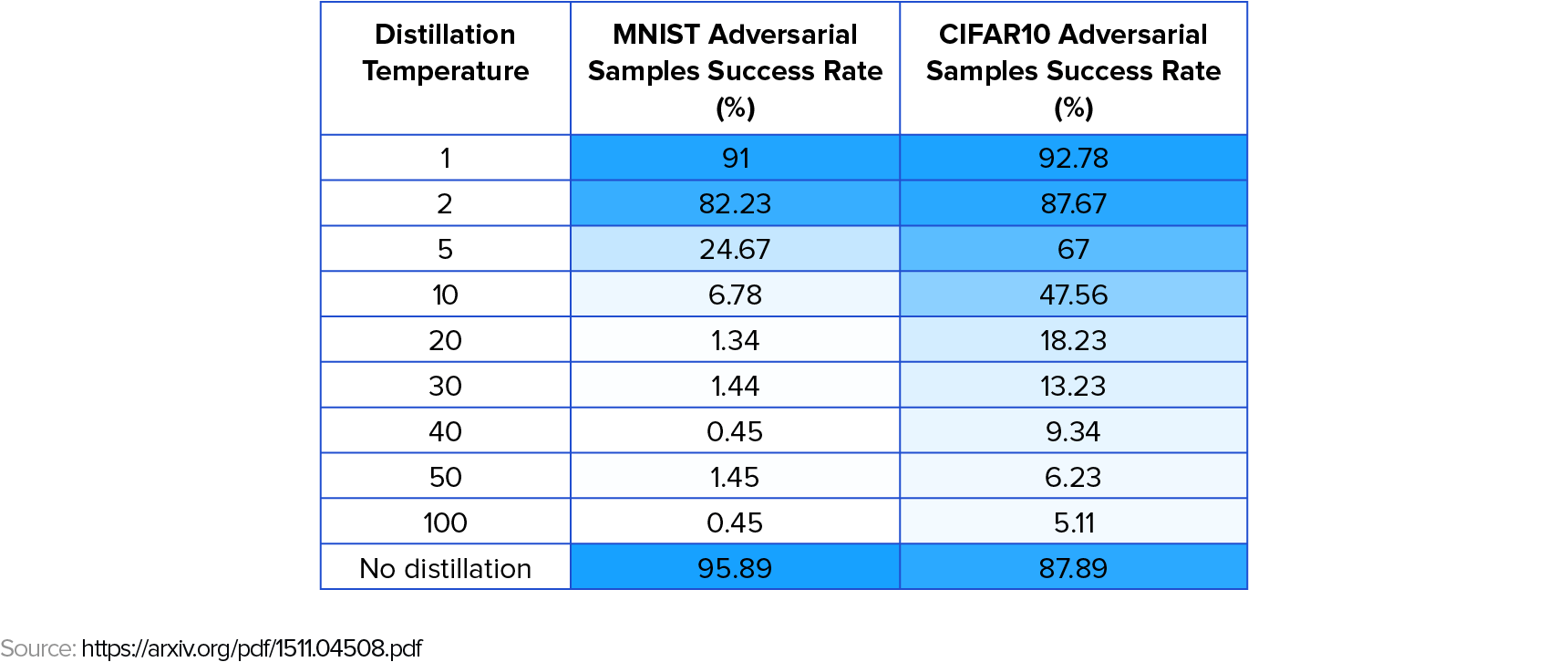
Defensive distillation successfully protects the network against the set of attacks attempted in Distillation as a Defense to Adversarial Perturbations against Deep Neural Networks.

Unfortunately, a later paper by University of California, Berkeley reserachers presented a new set of attack methods that defeat defensive distillation. These attacks are improvements over the L-BFGS method that prove that defensive distillation is not a general solution against adversarial examples.
Adversarial Training
Nowadays, adversarial training is the most effective defense strategy. Adversarial examples are generated and used when training the model. Intuitively, if the model sees adversarial examples during training, its performance at prediction time will be better for adversarial examples generated in the same way.
Ideally, we would like to employ any known attack method to generate adversarial examples during training. However, for a big dataset with high dimensionality (like ImageNet) robust attack methods like L-BFGS and the improvements described in the Berkeley paper are too computationally costly. In practice, we can only afford to use a fast method like FGS or iterative FGS can be employed.
Adversarial training uses a modified loss function that is a weighted sum of the usual loss function on clean examples and a loss function from adversarial examples.
During training, for every batch of $m$ clean images we generate $k$ adversarial images using the current state of the network. We forward propagate the network both for clean and adversarial examples and compute the loss with the formula above.
An improvement to this algorithm presented in this conference paper is called ensemble adversarial training. Instead of using the current network to generate adversarial examples, several pre-trained models are used to generate adversarial examples. On ImageNet, this method increases the robustness of the network to black-box attacks. This defense was the winner of the 1st round in the NIPS 2017 competition on Defenses against Adversarial Attacks.
Conclusions and Further Steps
As of today, attacking a machine learning model is easier than defending it. State-of-the art models deployed in real-world applications are easily fooled by adversarial examples if no defense strategy is employed, opening the door to potentially critical security issues. The most reliable defense strategy is adversarial training, where adversarial examples are generated and added to the clean examples at training time.
If you want to evaluate the robustness of your image classification models to different attacks I recommend that you use the open-source Python library cleverhans. Many attack methods can be tested against your model, including the ones mentioned in this article. You can also use this library to perform adversarial training of your model and increase its robustness to adversarial examples.
Finding new attacks and better defense strategies is an active area of research. Both more theoretical and empirical work is required to make machine learning models more robust and safe in real-world applications.
I encourage the reader to experiment with these techniques and publish new interesting results. Moreover, any feedback regarding the present article is very welcome by the author.
Further Reading on the Toptal Blog:
Understanding the basics
What is an adversarial example?
An adversarial example is an input (e.g. image, sound) designed to cause a machine learning model to make a wrong prediction. It is generated from a clean example by adding a small perturbation, imperceptible for humans, but sensitive enough for the model to change its prediction.
What is an adversarial attack?
Any machine learning model used in a real-world scenario is subject to adversarial attacks. This includes computer vision models used in self-driving cars, facial recognition systems used in airports or the speech-recognition software in your cell phone assistant.
What is an adversarial attack?
An adversarial attack is a strategy aimed at causing a machine learning model to make a wrong prediction. It consists of adding a small and carefully designed perturbation to a clean image, that is imperceptible for the human eye, but that the model sees as relevant and changes its prediction.
Pau Labarta Bajo
Barcelona, Spain
Member since April 24, 2019
About the author
Pau has extensive experience in quantitative finance. He combines love of statistics and machine learning with excellent Python skills.
Expertise
PREVIOUSLY AT


