Supply Chain Optimization Using Python and Mathematical Modeling

Creating efficient supply chains is one of the greatest challenges of the 2020s—and not just because of the disruptions brought about by the COVID-19 pandemic. Supply chains were strained before the pandemic due to global bottlenecks and shortages in labor and equipment. To keep up with demand, market players must rapidly modernize business processes through digitization and intelligent planning.

My career as a developer and data science consultant is focused on heavy industry: rail, mining, oil and gas, shipping, and postal logistics. All of these sectors have been greatly impacted by supply chain issues over these last few years. In this piece, I explore how mathematical optimization modeling and Python can resolve a core challenge in the mining industry: satisfying customized demand and maximizing profit through product blending.

An Optimization Approach for the Modern Supply Chain

In the typical supply chain scenario, a supplier delivers a specific finished product to a customer. In our example, to accomplish this, a supplier must:

1. Gather the necessary components from multiple source locations (e.g., production sites, warehouses).
2. Combine the components, executing a specific procedure to create a finished good. In a mining supply chain, this is referred to as product blending.
3. Deliver the finished product to a single target location (e.g., the customer’s site).

Done right, product blending enables the supplier to maximize value by leveraging trade-offs between customer needs and the supply chain. Mathematical optimization modeling is the ideal solution for addressing product blending in combination with logistical challenges such as scheduling, planning, packing, and routing.

A graph theoretical approach, like network flow optimization, works efficiently for challenges with a clear restricted scope (e.g., asking Google Maps how to get from A to B). But to handle more intricate challenges that impact overlapping aspects of the supply chain (e.g., product blending), mixed-integer programming is a powerful framework. Fast, well-researched, and established, mixed-integer programming allows users to address the vast majority of scheduling, planning, and routing issues.

To model and solve supply chain problems, I recommend using Python and its open-source libraries due to their strong optimization communities.

Product Blending in a Mining Supply Chain

As an example of product blending, let’s consider a mining supply chain that comprises several mines and produces a variety of raw material components. Typically, these components have to be routed to seaports. To keep our example simple, we will connect to just one seaport via a rail network that also links the mines.

We’ll use the following terms:

Raw material components retrieved from mines are transported by rail to a port, with the customer vessel as the final destination. Depending on the designated port’s berthing schedule or other circumstances, temporary storage of the components at a stockpile may be necessary. At the port, the train will either deposit the load onto a stockpile or unload it directly onto the customer vessel (what we call a direct hit).

Components are stored at mines and seaports. Mines are normally established in remote locations where storage space is cheap and plentiful. Ports, on the other hand, exist in industrial areas that usually have limited space, making port stockpiles expensive to use.

Modeling Details

Our hypothetical customer has demanded product blends that consist of different components. These blends must conform to the relevant mineral property standards, as defined by the customer (e.g., CSR value). To illustrate how this model would be built, let’s say that we have three mines that produce seven components, as follows:

The letter in a component’s name indicates the component’s source mine (e.g., component A3 was sourced at Mine A). Let’s agree that components that share a number are similar and as such, we may treat them equivalently: For example, A1, B1, and C1 are essentially the same type of raw material.

All components are transported by rail to the port, where we can either perform a direct hit or deposit each component at a suitable stockpile. Space limitations may prohibit us from storing components individually. As such, when blending a product, we may not have access to each component separately and may need to extract several components from a single stockpile simultaneously.

Now, let’s discuss the blending rules that customers typically demand for their products.

Product Blending Rules

Customers routinely ask for a blend of components per customer-specific rules on both how a blend may be performed and which spec assays are necessary. Such rules fall into two categories, component blending rules and spec blending rules.

Notice that, typically, the deviation penalty amount increases as a linear function as the boundary violation grows:

The optimization of blending includes trade-offs between accepting penalties for spec blending and the availability of components.

Mathematical Modeling for Extraction

When creating a product blending model, we must choose between different extraction types. For blending, average extraction is the most common extraction type. In average extraction, we model based on an assumption that all components in the stockpile are thoroughly mixed together. Layered extraction, where we model using a last-in, first-out rule, is an alternative to using average extraction:

The idea of layered extraction may be appealing, as it closely simulates the reality of the storing logistics at most stockpiles. However, from a mathematical modeling perspective, average extraction is preferred for computational reasons. The decision to use layered extraction should be carefully evaluated by business professionals and engineers to avoid introducing unnecessary complications into a modeling approach.

When using average extraction, the proportions of extracted components to one another are identical to those of the unextracted components. For example, average extraction says that an extraction from stockpile X containing 75% of component A3 and 25% of component C4 contains the same components and the same proportions as stockpile X in its entirety.

When layered extraction is used, the proportions of extracted components to one another are rarely, if ever, identical to those of the unextracted components. Layered extraction says that, for example, an extraction from stockpile X would not necessarily contain the same components as stockpile X in its entirety, nor the same proportions as stockpile X. This is because we would be extracting whatever component(s) are at the top of the stockpile (last-in, first-out).

The inconsistent nature of a layered extraction makes it difficult to model loading variables. Therefore, average extraction, which avoids complex interdependencies between the loading variables, is the preferred option when layered extraction is not a business requirement (see also “Coding to Solve Product Blending”).

Product Blending Modeling

Let’s consider the case of average extraction. Say we would like to monitor and model components deposited at a stockpile or customer vessel. Here are three possible extraction and modeling scenarios:

Scenario 1: Single Extraction Modeling We can extract any/all components, regardless of type. In this example, we may treat component A1 (sourced at Mine A) and B1 (sourced at Mine B) as if they are the same component because they are similar enough.
Scenario 2: Product Blend Extraction Modeling We can extract a feasible product blend. In this example, the extracted product blend conforms to the customer’s product blending rule requirements: The ratios of components A2, B2, and C1 at Port Stockpile 2 adhere to the customer’s component blending rules. In addition, the components’ spec assays adhere to the customer’s spec blending rules.
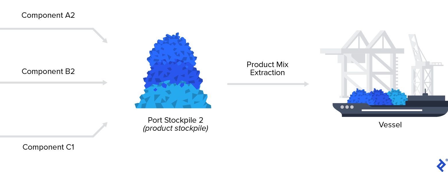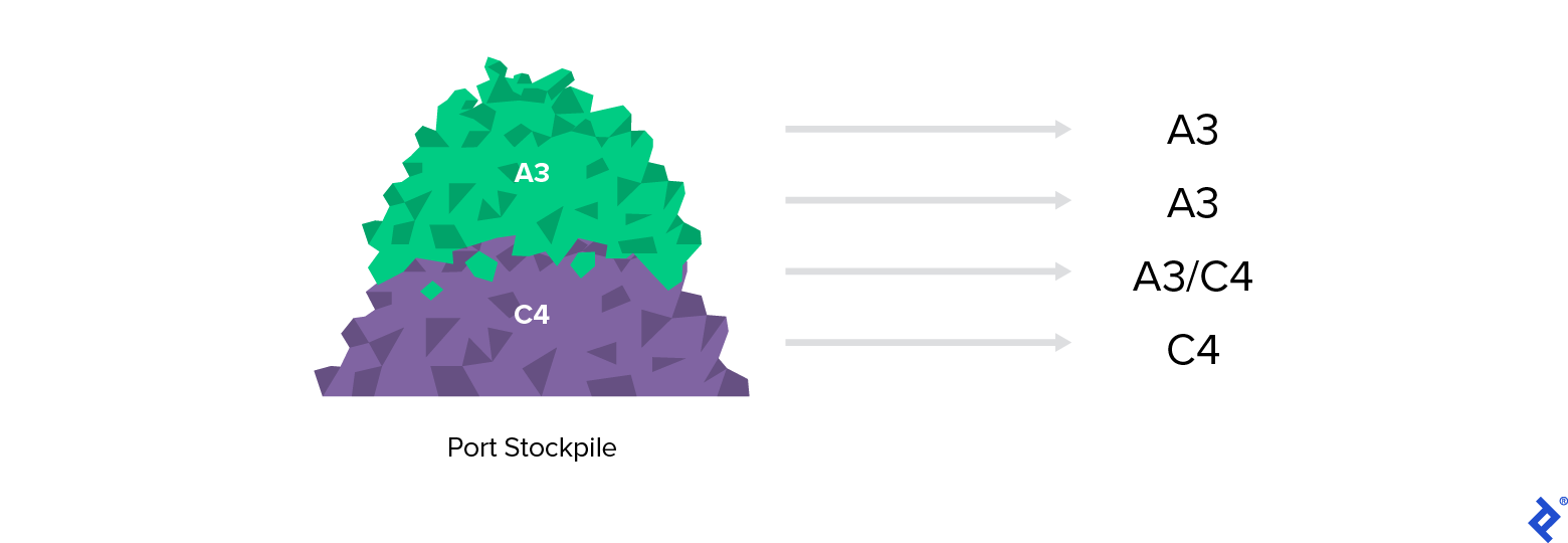
Scenario 3: Flexible Mix Extraction Modeling We can only extract an invalid component mix that does not conform to the customer’s component blending rules and thus does not form a product on its own. In this example, since our blend of components A3 and C4 does not form a valid product, we can: Await the arrival of and combine the necessary components. Combine the blend with other stockpile(s). Load the blend directly onto a customer vessel to be combined with another blend.

From a modeling perspective, I recommend creating mixed-integer programming formulations to address product blending. We can model product blending by using only real-valued variables and linear constraints, making it relatively easy to calculate and monitor blends.

Things can get complicated when product blending modeling overlaps with scheduling decisions that require binary variables for modeling purposes, such as decisions around vessel berthing or train schedules.

Coding to Solve Product Blending

Python is ideal for coding and solving mixed-integer programming formulations. Use the PuLP library to formulate supply chain problems, such as defining variables, constraints, and objective functions. Conveniently, PuLP’s syntax closely resembles a clean mathematical formulation.

You can then integrate an open-source solver like Cbc or, if your budget allows, a commercial solver like Gurobi or CPLEX. The commercial options provide a tremendous performance boost compared to Cbc.

The following pseudocode examples demonstrate how we define loading variables and constraints. The loading variables are:

load[v=vessel, p=port, c=component, prd=product, t=time]

These variables have five indices: vessel, port, component, product, and time. In practice, you will define many more types of loading variables.

Adding a product index to the loading variables is useful for tracking the specific product for which a component is designated. Since loading variables are real values (as opposed to integers), they do not pose a big computational challenge. Component blending rules can now be modeled as follows:

load[v, p, A2, prd, t] >= 0.5 * sum(load[v, p, c, prd, t] for all c that serve product prd of vessel v)
load[v, p, C1, prd, t] <= 0.2 * sum(load[v, p, c, prd, t] for all c that serve product prd of vessel v)
load[v, p, C1, prd, t] + load[v, p, B2, prd, t] <= 0.5 * sum(load[v, p, c, prd, t] for all c that serve product prd of vessel v)

Spec blending rules can be implemented with a similar linear approach. However, these constraints would be a bit more complicated, since spec assays are usually normalized by the loaded amount. While simpler to execute, direct modeling would introduce non-linearities and, thus, would be impractical. Instead, it would be better to calculate weighted pseudo-assay values and then reapply the linear equations. Caveat: The constraints may overlap with binary scheduling variables—but that discussion is beyond the scope of this article.

I wholeheartedly recommend incorporating blending rules into a supply chain model. My past clients have had consistent successes with optimized customer-specific blending, which increased the computational complexity of their scheduling models by only a hair.

Transforming Your Mining Supply Chain to Incorporate Blending

Product blending is strongly connected to rail and port operations, heavily impacting day-to-day decisions, such as where to transport which components or where to deposit and/or extract components.

The ideal digital state is a comprehensive scheduling tool that provides forward-looking recommendations for rail and port, with a blending optimization model integrated as a key part. When appropriate (e.g., to respond to changing weather conditions), ad hoc problem-solving by authorized rail and port operators can correct selected recommendations.

For each unique supply chain, a custom scheduling tool makes sense. Using an Agile process, we could identify the impact of product blending before our full digital tool is released. Close collaboration with operators and coordinators—at all times—would go a long way toward addressing any change management risks.

To structure and code the models necessary for building a scheduling application, engage the talents of data scientists, data engineers, and optimization experts. In today’s challenging and competitive environment, businesses that implement product blending stay ahead of the competition.

The editorial team of the Toptal Engineering Blog extends its gratitude to John Lee for reviewing the code samples and other technical content presented in this article.