Business Intelligence Platform: Tutorial Using MongoDB Aggregation Pipeline
In today’s data-driven world, researchers are busy answering interesting questions by churning through huge volumes of data. Some obvious challenges they face are due to the sheer size of the dataset they have to deal with. In this article, we take a peek at a simple business intelligence platform implemented on top of the MongoDB Aggregation Pipeline.
In today’s data-driven world, researchers are busy answering interesting questions by churning through huge volumes of data. Some obvious challenges they face are due to the sheer size of the dataset they have to deal with. In this article, we take a peek at a simple business intelligence platform implemented on top of the MongoDB Aggregation Pipeline.
Avinash is a senior developer with experience designing & developing data visualizations.
PREVIOUSLY AT

Using data to answer interesting questions is what researchers are busy doing in today’s data driven world. Given huge volumes of data, the challenge of processing and analyzing it is a big one; particularly for statisticians or data analysts who do not have the time to invest in learning business intelligence platforms or technologies provided by Hadoop eco-system, Spark, or NoSQL databases that would help them to analyze terabytes of data in minutes.
The norm today is for researchers or statisticians to build their models on subsets of data in analytics packages like R, MATLAB, or Octave, and then give the formulas and data processing steps to IT teams who then build production analytics solutions.
One problem with this approach is that if the researcher realizes something new after running his model on all of the data in production, the process has to be repeated all over again.
What if the researcher could work with a MongoDB developer and run his analysis on all of the production data and use it as his exploratory dataset, without having to learn any new technology or complex programming languages, or even SQL?

If we use MongoDB’s Aggregation Pipeline and MEAN effectively we can achieve this in a reasonably short time. Through this article and the code that is available here in this GitHub repository, we would like to show how easy it is to achieve this.
Most of the Business Intelligence tools that are on the market are providing ways for researchers to import datasets from NoSQL and other Big Data technologies into the tool, then the transformations and analysis are done inside the tool. But in this business intelligence tutorial we are using the power of MongoDB Aggregation Pipeline without pulling the data out of MongoDB, and the researcher is using a simple interface to do all kinds of transformations on a production big data system.
MongoDB Aggregation Pipeline for Business Intelligence
Simply put, MongoDB’s aggregation pipeline is a framework to perform a series of data transformations on a dataset. The first stage takes the entire collection of documents as input, and from then on each subsequent stage takes the previous transformation’s result set as input and produces some transformed output.
There are 10 types of transformations that can be used in an aggregation pipeline:
-
$geoNear: outputs documents in order of nearest to farthest from a specified point
-
$match: filters input record set by any given expressions
-
$project: creates a resultset with a subset of input fields or computed fields
-
$redact: restricts the contents of the documents based on information from the document
-
$unwind: takes an array field with n elements from a document and returns n documents with each element added to each document as a field replacing that array
-
$group: groups by one or more columns and perform aggregations on other columns
-
$limit: picks first n documents from input sets (useful for percentile calculations, etc.)
-
$skip: ignores first n documents from input set
-
$sort: sorts all input documents as per the object given
-
$out: takes all the documents returned from previous stage and writes them to a collection
Except for the first and last in the list above, there are no rules about the order in which these transformations may be applied. $out should be used only once, and at the end, if we want to write the result of the aggregation pipeline to a new or existing collection. $geoNear can be used only as the first stage of a pipeline.
In order to make things easier to understand, let us walk through two datasets and two questions relevant to these datasets.
Difference in Salaries by Designation
In order to explain the power of MongoDB’s aggregation pipeline, we have downloaded a dataset which has salary information of university instructional staff for the entire US. This data is available at nces.ed.gov. We have data from 7598 institutions with the following fields:
var FacultySchema = mongoose.Schema({
	InstitutionName : String,
	AvgSalaryAll : Number,
	AVGSalaryProfessors : Number,
	AVGSalaryAssociateProfessors : Number,
	AVGSalaryAssistantProfessors : Number,
	AVGSalaryLecturers : Number,
	AVGSalaryInstructors : Number,
	StreetAddress : String,
	City : String,
	State : String,
	ZIPCode : String,
	MenStaffCount : Number,
	WomenStaffCount : Number
}
With this data we want to find out (on average) what the difference is between salaries of associate professors and professors by state. Then, an associate professor can realize in which state he is valued closer to a professor in terms of salary.
To answer this question, a researcher first needs to weed out bad data from the collection, because there are a few rows/documents in our dataset where the average salary is a null or empty string. To accomplish this cleaning of the dataset we will add the following stage:
{$match: {AVGSalaryProfessors: {$not: {$type: 2}}, AVGSalaryAssociateProfessors: {$not: {$type: 2}}}}
This will filter out all the entities which have string values in those two fields. In MongoDB, each type is represented with a unique number - for strings, the type number is 2.
This dataset is a good example because in real world data analytics, engineers often have to deal with data cleanups as well.
Now that we have some stable data, we can continue to the next stage where we will average the salaries by state:
{$group: {_id: "$State", StateAVGSalaryProfessors: {$avg: "$AVGSalaryProfessors"}, StateAVGSalaryAssociateProfessors: {$avg: "$AVGSalaryAssociateProfessors"}}}
We just need to run a projection of the above result set and get the difference in state average salaries, as shown below in Stage 3 of our pipeline:
{$project: {_ID: 1, SalaryDifference: {$subtract: ["$StateAVGSalaryProfessors", "$StateAVGSalaryAssociateProfessors"]}}}
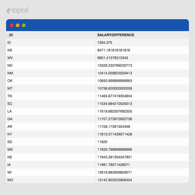
This should give us the state level average salary difference between professors and associate professors from a dataset of 7519 educational institutions all over US. To make it even more convenient to interpret this information, let us do a simple sort so we know which state has the least difference by adding a $sort stage:
{$sort: { SalaryDifference: 1}}
From this dataset, it is apparent that Idaho, Kansas, and West Virginia are three states where the difference in salaries of associate professors and professors is the least compared to all the other states.
The full aggregation pipeline generated for this is shown below:
[
{$match: {AVGSalaryProfessors: {$not: {$type: 2}}, AVGSalaryAssociateProfessors:  {$not: {$type: 2}}}},
{$group: {_id: "$State", StateAVGSalaryProfessors: {$avg: "$AVGSalaryProfessors"}, StateAVGSalaryAssociateProfessors: {$avg: "$AVGSalaryAssociateProfessors"}}},
{$project: {_ID: 1, SalaryDifference: {$subtract: ["$StateAVGSalaryProfessors", "$StateAVGSalaryAssociateProfessors"]}}},
{$sort: { SalaryDifference: 1}}
]
The resulting dataset that shows up looks like this. Researchers can also export these results to CSV in order to report on it using visualization packages like Tableau, or through simple Microsoft Excel charts.

Average Pay by Employment Type
Another example that we will explore in this article involves a dataset obtained from www.data.gov. Given the payroll information of all state and local government organizations in the United States of America, we would like to figure out the average pay of full-time and part-time “Financial Administration” employees in each state.
The dataset has been imported, resulting in 1975 documents where each document follows this schema:
mongoose.Schema({
	State : String,
	GovernmentFunction : String,
	FullTimeEmployees : Number,
	VariationPCT : Number,
	FullTimePay : Number,
	PartTimeEmployees : Number,
	PartTimePay : Number,
	PartTimeHours : Number,
	FullTimeEquivalentEmployment : Number,
	TotalEmployees : Number,
	TotalMarchPay : Number
	}, {collection: 'payroll'});
The answer to this question may help a Financial Administration employee to choose the best state to move to. With our MongoDB aggregator pipeline based tool, this can be done quite easily:
In the first stage, filter on GovernmentFunction column to discard all non-”Financial Administration” entities:
{$match:{GovernmentFunction:'Financial Administration'}}
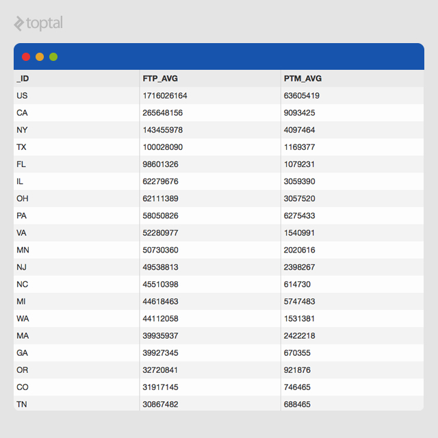
In the next stage of the tutorial, we will group the entities by state and calculate the average full time and part time salaries in each state:
{$group: {_id: '$State', FTP_AVG: {$avg: '$FullTimePay'}, PTM_AVG: {$avg: '$PartTimePay'}}}
Finally, we will sort the results from higher paying states to lower paying states:
{$sort: {FTP_AVG: -1, PTM_AVG: -1}}
This should allow the tool to generate the following aggregation pipeline:
[
    {$match:{GovernmentFunction:'Financial Administration'}},
    {$group: {_id: '$State', FTP_AVG: {$avg: '$FullTimePay'}, PTM_AVG: {$avg: '$PartTimePay'}}},
    {$sort: {FTP_AVG: -1, PTM_AVG: -1}}
]
Running the aggregation pipeline should produce some results like this:

Building Blocks
To build this business intelligence application we used MEAN, which is a combination of MongoDB, ExpressJS, AngularJS, and NodeJS.

As you may already know, MongoDB is a schemaless document database. Even though each document that it stores is limited to 16MB in size, its flexibility and performance along with the aggregation pipeline framework it provides makes MongoDB a perfect fit for this tool. Getting started with MongoDB is very easy, thanks to its comprehensive documentation.
Node.js, another integral component of the MEAN, provides the event-driven server-side Javascript environment. Node.js runs Javascript using Google Chrome’s V8 engine. The scalability promises of Node.js is what is driving many organizations towards it.
Express.js is the most popular web application framework for Node.js. It makes it easy to build APIs or any other kind of server-side business layer for web applications. It is very fast because of its minimalist nature, but is also quite flexible.
AngularJS, created and maintained by a number of Google engineers, is rapidly becoming one of the most popular front-end Javascript frameworks available at our disposal.
There are two reasons why MEAN is so popular and our choice for application development at techXplorers:
-
The skillset is simple. An engineer who understands JavaScript is good to go on all layers.
-
Communication between front-end to business to database layers all happens through JSON objects, which saves us significant time in design and development at different layers.
Conclusion
In this MongoDB aggregation pipeline tutorial we have demonstrated a cost effective way to give researchers a tool where they can use production data as exploratory datasets and run different sets of transformations to analyze and construct models from.
We were able to develop and deploy this application end-to-end in just 3 days. This applicaton was developed by a team of 4 experienced engineers (2 in the US and 2 in India) and a designer and freelance UX expert helping us with some thoughts on interface design. At some point in the future, I will take the time to explain how this level of collaboration works to build awesome products in unbelievably short time.
We hope you take advantage of MongoDB’s Aggregation Pipeline, and put power in the hands of your researchers who can change the world with their clever analysis and insights.
This application is live to be played with here.
Further Reading on the Toptal Blog:
Avinash Kaza
Leesburg, VA, United States
Member since November 6, 2013
About the author
Avinash is a senior developer with experience designing & developing data visualizations.
PREVIOUSLY AT


