Do the Math: Scaling Microservices Applications With Orchestrators
Automatically scaling container deployments in a microservices-based app architecture is downright luxurious…once it’s set up. But what’s the best way to tune an app’s orchestration parameters?
Automatically scaling container deployments in a microservices-based app architecture is downright luxurious…once it’s set up. But what’s the best way to tune an app’s orchestration parameters?
Antoine has done DevOps for microservice architectures since Docker was in beta and helped design the ecosystem for Cryptobox.
Expertise
It’s not quite a surprise that the microservices application architecture continues to invade software design. It is much more convenient to distribute the load, create highly-available deployments, and manage upgrades while easing development and team management.
But the story surely isn’t the same without container orchestrators.
It’s easy to want to use all of their key features, especially auto-scaling. What a blessing it is, watching container deployments fluctuating all day long, gently sized to handle the current load, freeing up our time for other tasks. We’re proudly satisfied of what our container monitoring tools are showing; meanwhile, we’ve just configured a couple of settings—yes, that’s (almost) all it took to create the magic!
That isn’t to say there is no reason to be proud of this: We are sure that our users are having a good experience, and that we are not wasting any money with oversized infrastructure. This is already quite considerable!
And of course, what a journey it was to get there! Because even if at the end there are not that many settings that need to be configured, it is a lot trickier than we usually might think before we can get started. Min/max number of replicas, upscale/downscale thresholds, sync periods, cool down delays—all those settings are very much tied together. Modifying one will most likely affect another, but you still have to arrange a balanced combination that will suit both your application/deployment and your infrastructure. And yet, you will not find any cookbook or any magic formula on the Internet, as it highly depends on your needs.
Most of us first set them to “random” or default values which we adjust afterward according to what we find while monitoring. That got me thinking: What if we were able to establish a more “mathematical” procedure that would help us find the winning combination?
Calculating Container Orchestration Parameters
When we think about auto-scaling microservices for an application, we are actually looking at improving on two major points:
- Making sure the deployment can scale up fast in the case of a rapid load increase (so users don’t face timeouts or HTTP 500s)
- Lowering the cost of the infrastructure (i.e., keeping instances from being under-loaded)
This basically means optimizing the container software thresholds for scaling up and scaling down. (Kubernetes’ algorithm has a single parameter for the two).
I will show later that all of the instance-related parameters are tied to the upscale-threshold. This is the most difficult one to calculate—hence this article.
Note: Regarding parameters that are set cluster-wide, I don’t have any good procedure for them, but at the end of this article, I will introduce a piece of software (a static web page) that takes them into account while calculating an instance’s auto-scaling parameters. That way, you will be able to vary their values to consider their impact.
Calculating the Scale-up Threshold
For this method to work, you have to make sure that your application meets the following requirements:
- The load has to be evenly distributed across every instance of your application (in a round-robin manner)
- Request timings must be shorter than your container cluster’s load-check interval.
- You have to consider running the procedure on a great number of users (defined later).
The main reason for those conditions comes from the fact that the algorithm does not calculate the load as being per user but as a distribution (explained later).
Getting All Gaussian
First we have to formulate a definition for a rapid load increase or, in other words, a worst-case scenario. To me, a good way to translate it is: having a great number of users performing resource-consuming actions within a short period of time—and there’s always the possibility that it happens while another group of users or services are performing other tasks. So let’s start from this definition and try to extract some math. (Get your aspirin ready.)
Introducing some variables:
- $N_{u}$, the “great number of users”
- $L_{u}(t)$, the load generated by a single user performing the “resource-consuming operation” ($t=0$ points to the moment when the user starts the operation)
- $L_{tot}(t)$, the total load (generated by all users)
- $T_{tot}$, the “short period of time”
In the mathematical world, talking about a great number of users performing the same thing at the same time, users’ distribution over time follows a Gaussian (or normal) distribution, whose formula is:
\[G(t) = \frac{1}{\sigma \sqrt{2 \pi}} e^{\frac{-(t-\mu)^2}{2 \sigma^2}}\]Here:
- µ is the expected value
- σ is the standard deviation
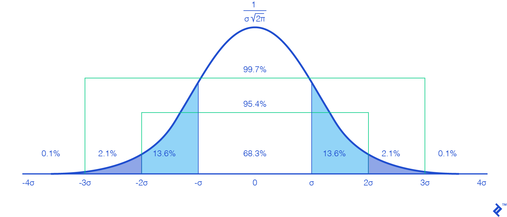
And it’s graphed as follows (with $µ=0$):

Probably reminiscent of some classes you’ve taken—nothing new. However, we do face our first issue here: To be mathematically accurate, we would have to consider a time range from $-\infty$ to $+\infty$, which obviously cannot be computed.
But looking at the graph, we notice that values outside the interval $[-3σ, 3σ]$ are very close to zero and do not vary much, meaning their effect is really negligible and can be put aside. This is more so true, since our goal is to test scaling up our application, so we are looking for variations of large numbers of users.
Plus, since the interval $[-3σ, 3σ]$ contains 99.7 percent of our users, it is close enough to the total to work on it, and we just need to multiply $N_{u}$ by 1.003 to make up for the difference. Selecting this interval gives us $µ=3σ$ (since we are going to work from $t=0$).
Regarding the correspondence to $T_{tot}$, choosing it to be equal to $6σ$ ($[-3σ, 3σ]$) won’t be a good approximation, since 95.4 percent of users are in the interval $[-2σ, 2σ]$, which lasts $4σ$. So choosing $T_{tot}$ to be equal to $6σ$ will add half the time for only 4.3 percent of users, which is not really representative. Thus we choose to take $T_{tot}=4σ$, and we can deduce:
\(σ=\frac{T_{tot}}{4}\) and \(µ=\frac{3}{4} * T_{tot}\)
Were those values just pulled out of a hat? Yes. But this is what their purpose is, and this won’t affect the mathematical procedure. Those constants are for us, and defines notions related to our hypothesis. This only means that now that we have them set, our worst case scenario can be translated as:
The load generated by 99.7 percent of $N{u}$, performing a consuming operation $L{u}(t)$ and where 95.4 percent of them are doing it within the duration $T{tot}$.
(This is something worth remembering when using the web app.)
Injecting previous results into the user distribution function (Gaussian), we can simplify the equation as follows:
\[G(t) = \frac{4 N_{u}}{T_{tot} \sqrt{2 \pi}} e^\frac{-(4t-3T_{tot})^2}{T_{tot}^2}\]From now on, having $σ$ and $µ$ defined, we will be working on the interval $t \in [0, \frac{3}{2}T_{tot}]$ (lasting $6σ$).
What’s the Total User Load?
The second step in auto-scaling microservices is calculating $L_{tot}(t)$.
Since $G(t)$ is a distribution, to retrieve the number of users at a certain point in time, we have to calculate its integral (or use its cumulative distribution function). But since not all users start their operations at the same time, it would be a real mess trying to introduce $L_{u}(t)$ and reduce the equation to a usable formula.
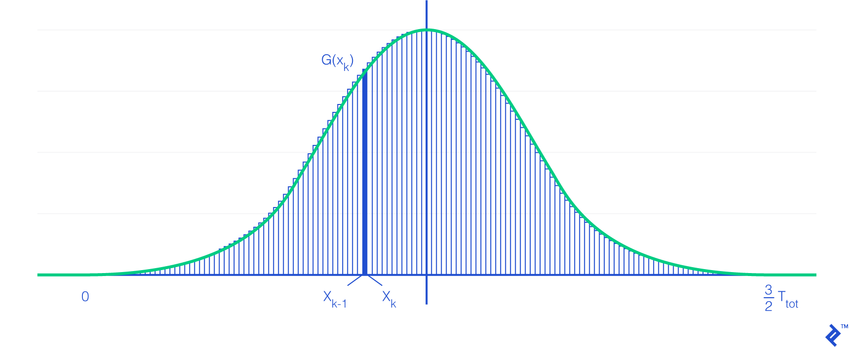
So to make this easier, we will be using a Riemann sum, which is a mathematical way to approximate an integral using a finite sum of small shapes (we will be using rectangles here). The more shapes (subdivisions), the more accurate the result. Another benefit of using subdivisions comes from the fact that we can consider all users within a subdivision to have started their operations at the same time.
Back to the Riemann sum, it has the following property connecting with integrals:
\[\int_{a}^{b} f( x )dx = \lim_{n \rightarrow \infty } \sum_{k=1}^{n} ( x_{k} - x_{k-1} )f( x_{k} )\]With $x_k$ defined as follows:
\[x_{ k } = a + k\frac{ b - a }{ n }, 0 \leq k \leq n\]This is true where:
- $n$ is the number of subdivisions.
- $a$ is the lower bound, here 0.
- $b$ is the higher bound, here $\frac{3}{2}*T_{tot}$.
- $f$ is the function—here $G$—to approximate its area.

Note: The number of users present in a subdivision is not an integer. This is the reason for two of the prerequisites: Having a great number of users (so the decimal part is not too impacting), and the need for the load to be evenly distributed across every instance.
Also note that we can see the rectangular shape of the subdivision on the right-hand side of the Riemann sum definition.
Now that we have the Riemann sum formula, we can say that the load value at time $t$ is the sum of every subdivision’s number of users multiplied by the user load function at their corresponding time. This can be written as:
\[L_{ tot }( t ) = \lim_{n \rightarrow \infty} \sum_{ k=1 }^{ n } ( x_{k} - x_{k-1} )G( x_{k} )L_{ u }( t - x_{k} )\]After replacing variables and simplifying the formula, this becomes:
\[L_{ tot }( t ) = \frac{6 N_{u}}{\sqrt{2 \pi}} \lim_{n \rightarrow \infty} \sum_{ k=1 }^{ n } (\frac{1}{n}) e^{-{(\frac{6k}{n} - 3)^{2}}} L_{ u }( t - k \frac{3 T_{tot}}{2n} )\]And voilà! We created the load function!
Finding the Scale-up Threshold
To finish, we just need to run a dichotomy algorithm which varies the threshold to find the highest value where the load per instance never exceeds its maximum limit all over the load function. (This is what is done by the app.)
Deducing Other Orchestration Parameters
As soon as you have found your scale-up threshold ($S_{up}$), other parameters are quite easy to calculate.
From $S_{up}$ you will know your maximum number of instances. (You can also look for the maximum load on your load function and divide per the maximum load per instance, rounded up.)
The minimum number ($N_{min}$) of instances has to be defined according to your infrastructure. (I would recommend having a minimum of one replica per AZ.) But it also needs to take into account the load function: As a Gaussian function increases quite rapidly, the load distribution is more intense (per replica) at the beginning, so you may want to increase the minimum number of replicas to cushion this effect. (This will most likely increase your $S_{up}$.)
Finally, once you have defined the minimum number of replicas, you can calculate the scale-down threshold ($S_{down}$) considering the following: As scaling down a single replica has no more effect on other instances than when scaling down from $N_{min}+1$ to $N_{min}$, we have to make sure the scale-up threshold will not be triggered right after scaling down. If it’s allowed to, this will have a yo-yo effect. In other words:
\[( N_{ min } + 1) S_{ down } < N_{ min }S_{ up }\]Or:
\[S_{ down } < \frac{N_{ min }}{N_{min}+1}S_{ up }\]Also, we can admit that the longer your cluster is configured to wait before scaling down, the safer it is to set $S_{down}$ closer to the higher limit. Once again, you will have to find a balance that suits you.
Note that when using the Mesosphere Marathon orchestration system with its autoscaler, the maximum number of instances that can be removed at once from scaling down is tied to AS_AUTOSCALE_MULTIPLIER ($A_{mult}$), which implies:
What About the User Load Function?
Yes, that’s a bit of an issue, and not the easiest one to mathematically solve—if it’s even possible at all.
To workaround this issue, the idea is to run a single instance of your application, and increase the number of users performing the same task repeatedly until the server load reaches the maximum it got assigned (but not over). Then divide by the number of users and calculate the average time of the request. Repeat this procedure with every action you want to integrate into your user load function, add some timing, and there you are.
I am aware that this procedure implies considering that each user request has a constant load over its processing (which is obviously incorrect), but the mass of users will create this effect as each of them are not at the same processing step at the same time. So I guess this is an acceptable approximation, but it once again insinuates that you are dealing with a great number of users.
You can also try with other methods, like CPU flame graphs. But I think it will be very difficult to create an accurate formula that will link user actions to resource consumption.
Introducing the app-autoscaling-calculator
And now, for the small web app mentioned throughout: It takes as input your load function, your container orchestrator configuration, and some other general parameters and returns the scale-up threshold and other instance-related figures.
The project is hosted on GitHub, but it also has a live version available.
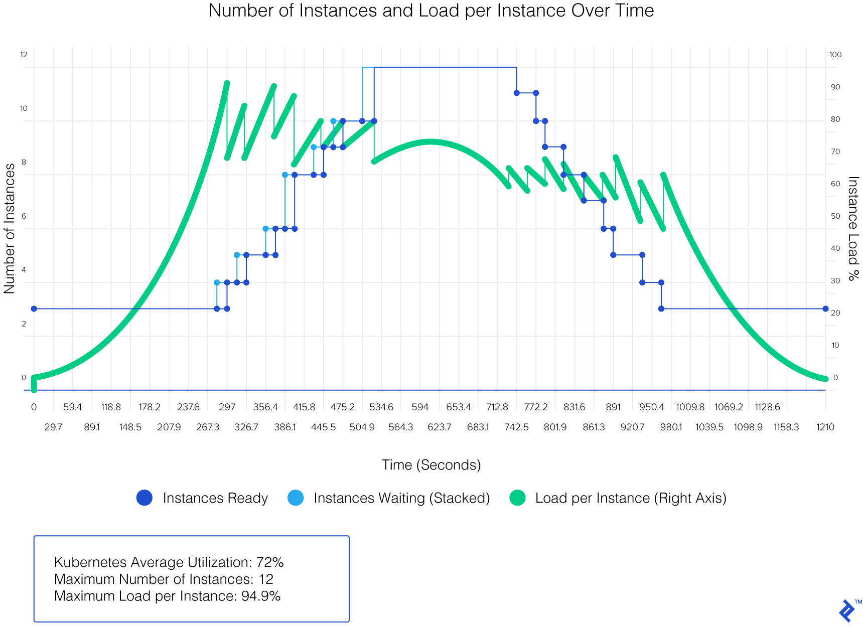
Here is the result given by the web app, run against the test data (on Kubernetes):

Scaling Microservices: No More Fumbling in the Dark
When it comes to microservices application architectures, container deployment becomes a central point of the whole infrastructure. And the better the orchestrator and containers are configured, the smoother the runtime will be.
Those of us in the field of DevOps services are always seeking better ways of tuning orchestration parameters for our applications. Let’s take a more mathematical approach to auto-scaling microservices!
Further Reading on the Toptal Blog:
Understanding the basics
How can you improve the scalability of a web application?
Using a microservices architecture is considered a best practice when it comes to maximizing scalability.
What does microservices architecture really mean?
Microservices are containerized components of an application that can be independently deployed.
Why do we need microservices architecture?
Besides making large applications easier to test and maintain, using a microservices application architecture is often the only way to allow for reliable, dynamic scaling. Furthermore, scaling microservices can be done automatically in response to user load.
What is container orchestration?
Container orchestration refers to coordinating microservices runtimes over a cluster of servers. One of its key features is the auto-scaling of applications.
Paris, France
Member since February 26, 2019
About the author
Antoine has done DevOps for microservice architectures since Docker was in beta and helped design the ecosystem for Cryptobox.

