Forecaster’s Toolbox: How to Perform Monte Carlo Simulations
One of the most important and challenging aspects of forecasting is handling the uncertainty inherent in examining the future. Every CEO, CFO, board member, investor, or investment committee member brings their own experience and approach to financial projections and uncertainty, influenced by different incentives. Oftentimes, comparing actual outcomes against projections underscores the need to explicitly recognize uncertainty.
Monte Carlo simulations are an extremely effective tool for handling risks and probabilities, used for everything from constructing DCF valuations, valuing call options in M&A, and discussing risks with lenders to seeking financing and guiding the allocation of VC funding for startups. This article provides a step-by-step tutorial on using Monte Carlo simulations in practice.
Stefan is the Director of Data-Driven Insights and Analytics for Cargotec, a leading provider of cargo and loading solutions. He has also served as an M&A director and a startup CFO, and led financial modeling and analysis as a leveraged finance manager at the Royal Bank of Scotland.
Expertise
PREVIOUSLY AT

Executive Summary
What Is a Monte Carlo Simulation?
- A Monte Carlo simulation in finance measures the probability of different outcomes in financial forecasts and estimates. They earn their name from the area of Monte Carlo in Monaco, famous for its high-end casinos. Random outcomes are central to the technique, just as they are to roulette and slot machines. Monte Carlo simulations are useful in a broad range of fields, including engineering, project management, oil & gas exploration and other capital-intensive industries, R&D, and insurance. This article focuses on applications in finance and business.
- Probability distributions. In the simulation, the uncertain inputs are described using probability distributions. When one or more inputs are described as probability distributions, the output also becomes a probability distribution. A computer randomly draws a number from each input distribution and calculates and saves the result. This is repeated hundreds or thousands of times, each called an iteration. When taken together, these iterations approximate the probability distribution of the final result.
Monte Carlo Simulation Tutorial
- Step 1: Choosing or Building the Model. Use a simple model, focused on highlighting the key features of using probability distributions. Note that, to start off, this model is no different from any other Excel model—the plugins work with your existing models and spreadsheets.
- Step 2: Creating the First Probability Distribution. First, we need to collect the information necessary for making our assumptions, then we need to choose the correct probability distributions to insert. It's important to note that the source of the key inputs/assumptions are the same regardless of which approach you take to handling uncertainty. Then you walk through and replace our key input values with probability distributions one by one. Next, you'll choose the distribution you want to use (e.g., normal).
- Step 3: Expanding the Revenue Forecast from One Year to Several. With Monte Carlo modeling, be mindful of how uncertainty and probability distributions stack on top of each other, such as over time. Another approach is to have five independent distributions, one for each year.
- Step 4: Expressing Margins as Probability Distributions. Here we can use the correlation functionality to simulate a situation where there is a clear correlation between relative market share and profitability, reflecting economies of scale. And depending on the time available, size of transaction, and other factors, it often makes sense to build an operating model and input the most uncertain variables explicitly. These include: product volumes and prices, commodity prices, FX rates, key overhead line items, monthly active users, and average revenue per unit (ARPU). It's also possible to model not only amounts variables such as development time, time to market, or market adoption rate.
- Step 5: Balance Sheet and Cash-flow Statement. Using the outlined approach, we can now continue through the balance sheet and cash flow statement, populating with assumptions and using probability distributions where it makes sense.
- Step 6: Finalizing the Model. Building a Monte Carlo model has one additional step compared to a standard financial model: The cells where we want to evaluate the results need to be specifically designated as output cells. The software will save the results of each iteration of the simulation for those cells for us to evaluate after the simulation is finished—all cells in the entire model are recalculated with each iteration, but the results of the iterations in other cells, which are not designated as input or output cells, are lost and cannot be analyzed after the simulation finishes. Once you have finished building the model it is time to run the simulation for the first time, by simply pressing "Start simulation" and waiting for a few seconds.
- Step 7: Interpreting the Results. We can now clearly see that there are a number of potential outcomes around that value, with different probabilities. This allows us to rephrase questions, such as "Will we hit our hurdle return rate with this investment?" to "How likely are we to hit or exceed our hurdle rate?" You can explore which outcomes are most likely, using for example a confidence interval. The visualization is helpful when communicating the results to different stakeholders, and you can overlay outputs from other transactions to visually compare how attractive and (un)certain the current one is compared to others.
- Toptal Finance can help you with all your modeling needs, with our Excel experts, financial modeling consultants, valuation specialists, and financial forecasting experts.
Introduction
First, the only certainty is that there is no certainty. Second, every decision as a consequence is a matter of weighing probabilities. Third, despite uncertainty we must decide and we must act. And lastly we need to judge decisions not only on the results, but how those decisions were made. – Robert E. Rubin
One of the most important and challenging aspects of forecasting is handling the uncertainty inherent in examining the future. Having built and populated hundreds of financial and operating models for LBOs, startup fundraisings, budgets, M&A, and corporate strategic plans since 2003, I have witnessed a wide range of approaches to doing so. Every CEO, CFO, board member, investor, or investment committee member brings their own experience and approach to financial projections and uncertainty—influenced by different incentives. Oftentimes, comparing actual outcomes against projections provides an appreciation for how large the deviations between forecasts and actual outcomes can be, and therefore the need for understanding and explicitly recognizing uncertainty.
I initially started out using scenario and sensitivity analyses to model uncertainty, and still consider them very useful tools. Since adding Monte Carlo simulations to my toolbox in 2010, I have found them to be an extremely effective tool for refining and improving how you think about risk and probabilities. I have used the approach for everything from constructing DCF valuations, valuing call options in M&A, and discussing risks with lenders to seeking financing and guiding the allocation of VC funding for startups. The approach has always been well received by board members, investors, and senior management teams. In this article, I provide a step-by-step tutorial on using a Monte Carlo simulation for forecasting by building a DCF valuation model.
Every Decision Is a Matter of Weighing Probabilities
Before starting with the case study, let’s review a few different approaches to handling uncertainty. The concept of expected value—the probability-weighted average of cash flows in all possible scenarios—is Finance 101. But finance professionals, and decision-makers more broadly, take very different approaches when translating this simple insight into practice. The approach can range from simply not recognizing or discussing uncertainty at all, on one hand, to sophisticated models and software on the other. In some cases, people end up spending more time discussing probabilities than calculating cash flows.
Aside from simply not addressing it, let’s examine a few ways of handling uncertainty in medium- or long-term projections. Many of these should be familiar to you.
|
Creating one scenario. This approach is the default for budgets, many startups, and even investment decisions. Besides not containing any information about the degree of uncertainty or recognition that outcomes may differ from the projections, it can be ambiguous and be interpreted differently according to the stakeholder. Some may interpret it as a stretch target, where the actual outcome is more likely to fall short than exceed. Some view it as a baseline performance with more upside than downside. Others may see it as a "Base Case" with 50/50 probability up and down. In some approaches, especially for startups, it is very ambitious and failure or shortfall is the more likely outcome by far, but a higher discount rate is used in an attempt to account for the risk. |
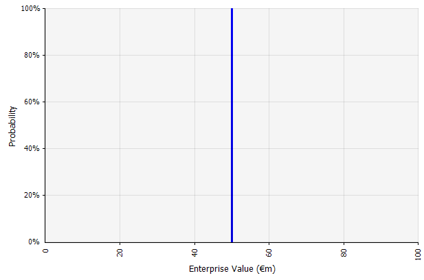 The inputs in the long-term cash-flow forecast under this approach are all point estimates, yielding a point estimate result of €50 million in this example, with an implicit probability of 100%. |
|
Creating multiple scenarios. This approach recognizes that reality is unlikely to unfold according to a single given plan.
|
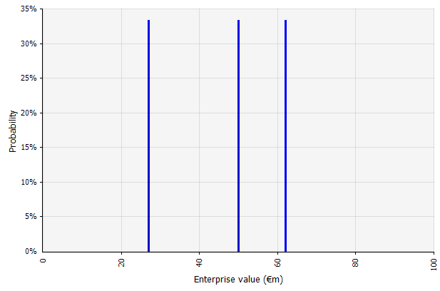 The three different scenarios yield three different results, here assumed to be equally likely. The probabilities of outcomes outside the high and low scenarios are not considered. |
|
Creating base-, upside, and downside cases with probabilities explicitly recognized. That is, the bear and bull cases contain, for example, a 25% probability in each tail, and the fair value estimate represents the midpoint. A useful benefit of this from a risk management perspective is the explicit analysis of tail risk, i.e., events outside the upside and downside scenarios. |
Illustration from the Morningstar Valuation Handbook 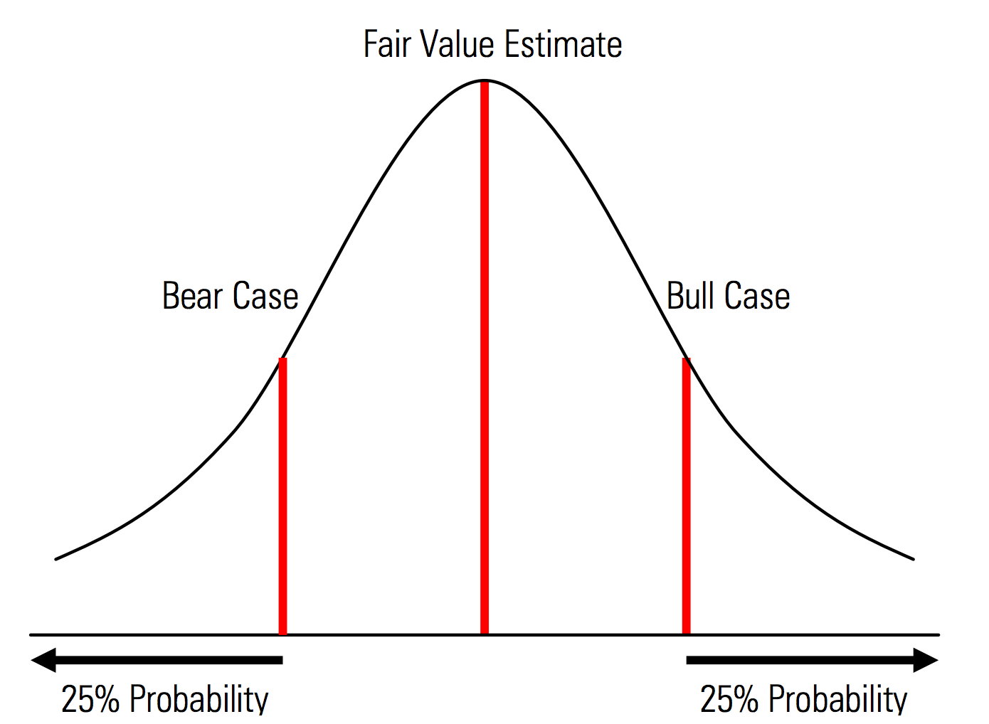 |
|
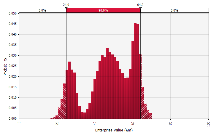
Using probability distributions and Monte Carlo simulations. Using probability distributions allows you to model and visualize the full range of possible outcomes in the forecast. This can be done not only at an aggregate level, but also for detailed individual inputs, assumptions, and drivers. Monte Carlo methods are then used to calculate the resulting probability distributions at an aggregate level, allowing for analysis of how several uncertain variables contribute to the uncertainty of the overall results. Perhaps most importantly, the approach forces everyone involved in the analysis and decision to explicitly recognize the uncertainty inherent in forecasting, and to think in probabilities. Just as the other approaches this has its drawbacks, including the risk of false precision and resulting overconfidence that may come with using a more sophisticated model, and the additional work required to select suitable probability distributions and estimate their parameters where otherwise only point estimates would be used. |
 |
What Is a Monte Carlo Simulation?
Monte Carlo simulations model the probability of different outcomes in financial forecasts and estimates. They earn their name from the area of Monte Carlo in Monaco, which is world-famous for its high-end casinos; random outcomes are central to the technique, just as they are to roulette and slot machines. Monte Carlo simulations are useful in a broad range of fields, including engineering, project management, oil & gas exploration and other capital-intensive industries, R&D, and insurance; here, I focus on applications in finance and business.
Probability Distributions
In the simulation, the uncertain inputs are described using probability distributions, described by parameters such as mean and standard deviation. Example inputs in financial projections could be anything from revenue and margins to something more granular, such as commodity prices, capital expenditures for an expansion, or foreign exchange rates.
When one or more inputs is described as probability distributions, the output also becomes a probability distribution. A computer randomly draws a number from each input distribution and calculates and saves the result. This is repeated hundreds, thousands, or tens of thousands of times, each called an iteration. When taken together, these iterations approximate the probability distribution of the final result.
Types of Inputs
The input distributions can be either continuous, where the randomly generated value can take any value under the distribution (for example a normal distribution), or discrete, where probabilities are attached to two or more distinct scenarios.
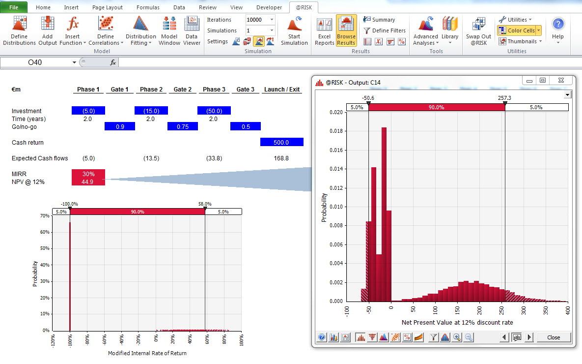
A simulation can also contain a mix of distributions of different types. Take, for example, a pharmaceutical R&D project with several stages that each have a discrete probability of success or failure. This can be combined with continuous distributions describing uncertain investment amounts needed for each stage and potential revenues if the project results in a product that reaches the market. The chart below shows the output from such a simulation: a ~65% probability of losing the entire investment of €5 million to €50 million (present value), and a ~35% probability of a net gain most likely in the range of €100 to €250—information that would be lost if key output metrics such as MIRR or NPV are shown as point estimates rather than probability distributions.
Monte Carlo Simulations in Practice
One reason Monte Carlo simulations are not more widely used is because typical finance day-to-day tools don’t support them very well. Excel and Google Sheets hold one number or formula result in each cell, and although they can define probability distributions and generate random numbers, building a financial model with Monte Carlo functionality from scratch is cumbersome. And, while many financial institutions and investment firms use Monte Carlo simulations for valuing derivatives, analyzing portfolios and more, their tools are typically developed in-house, proprietary or prohibitively expensive—rendering them inaccessible to the individual finance professional.
Thus, I want to draw attention to Excel plugins such as @RISK by Palisade, ModelRisk by Vose, and RiskAMP, which greatly simplify working with Monte Carlo simulations and allow you to integrate them within your existing models. In the following walkthrough, I will use @RISK.
Case study: Cash Flow Projections with Monte Carlo Simulation
Let us review a simple example that illustrates the key concepts of a Monte Carlo simulation: a five-year cash flow forecast. In this walkthrough, I set up and populate a basic cash flow model for valuation purposes, gradually replace the inputs with probability distributions, and finally run the simulation and analyze the results.
Step 1. Choosing or Building the Model
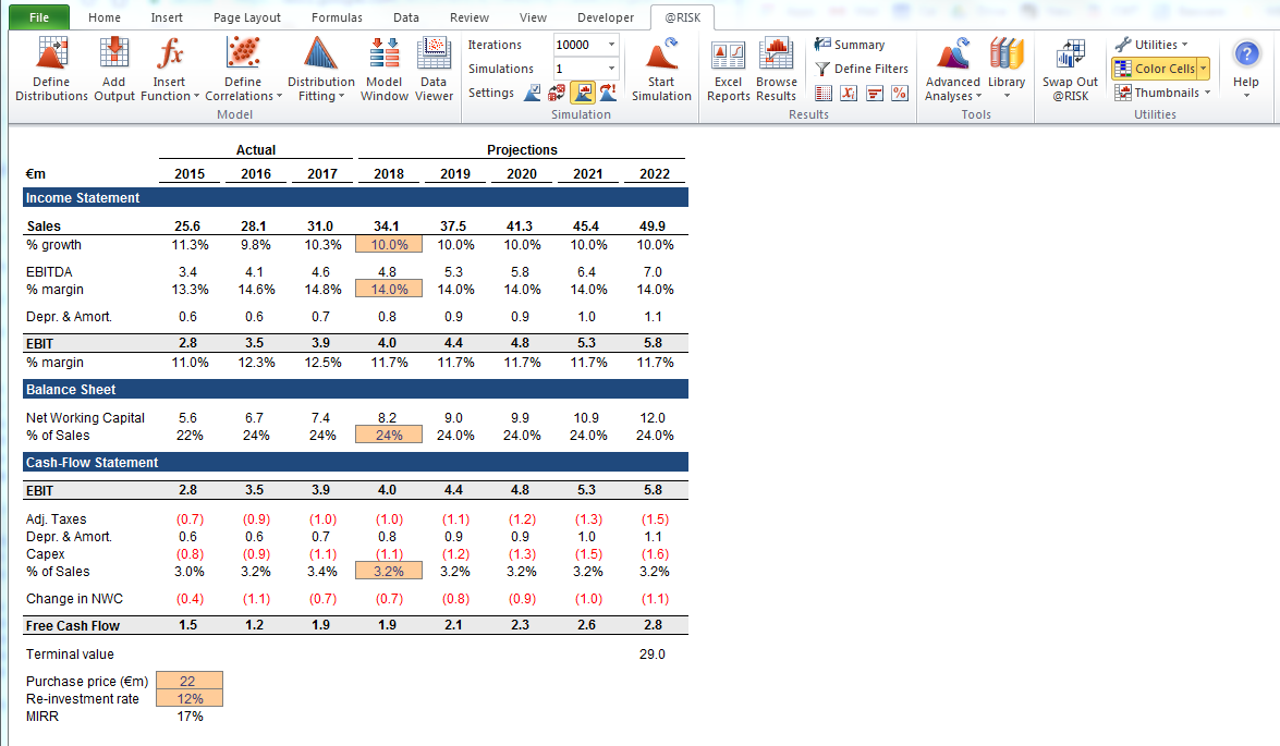
To start, I use a simple model, focused on highlighting the key features of using probability distributions. Note that, to start off, this model is no different from any other Excel model; the plugins I mentioned above work with your existing models and spreadsheets. The model below is a simple off-the-shelf version populated with assumptions to form one scenario.
Step 2. Creating the First Probability Distribution
First, we need to collect the information necessary for making our assumptions, then we need to choose the correct probability distributions to insert. It’s important to note that the source of the key inputs/assumptions are the same regardless of which approach you take to handling uncertainty. Commercial due diligence, a comprehensive review of the company’s business plan in the context of projected market development, industry trends, and competitive dynamics, typically includes extrapolation from historical data, incorporating expert opinion, conducting market research, and interviewing market participants. In my experience, experts and market participants are happy to discuss different scenarios, risks, and ranges of outcomes. However, most do not explicitly describe probability distributions.
Let us now walk through and replace our key input values with probability distributions one by one, starting with the estimated sales growth for the first forecast year (2018). The @RISK plugin for Excel can be evaluated with a 15-day free trial so you can download it from the Palisade website and install it with a few clicks. With the @RISK plugin enabled, select the cell you want the distribution in and select “Define distribution” in the menu.
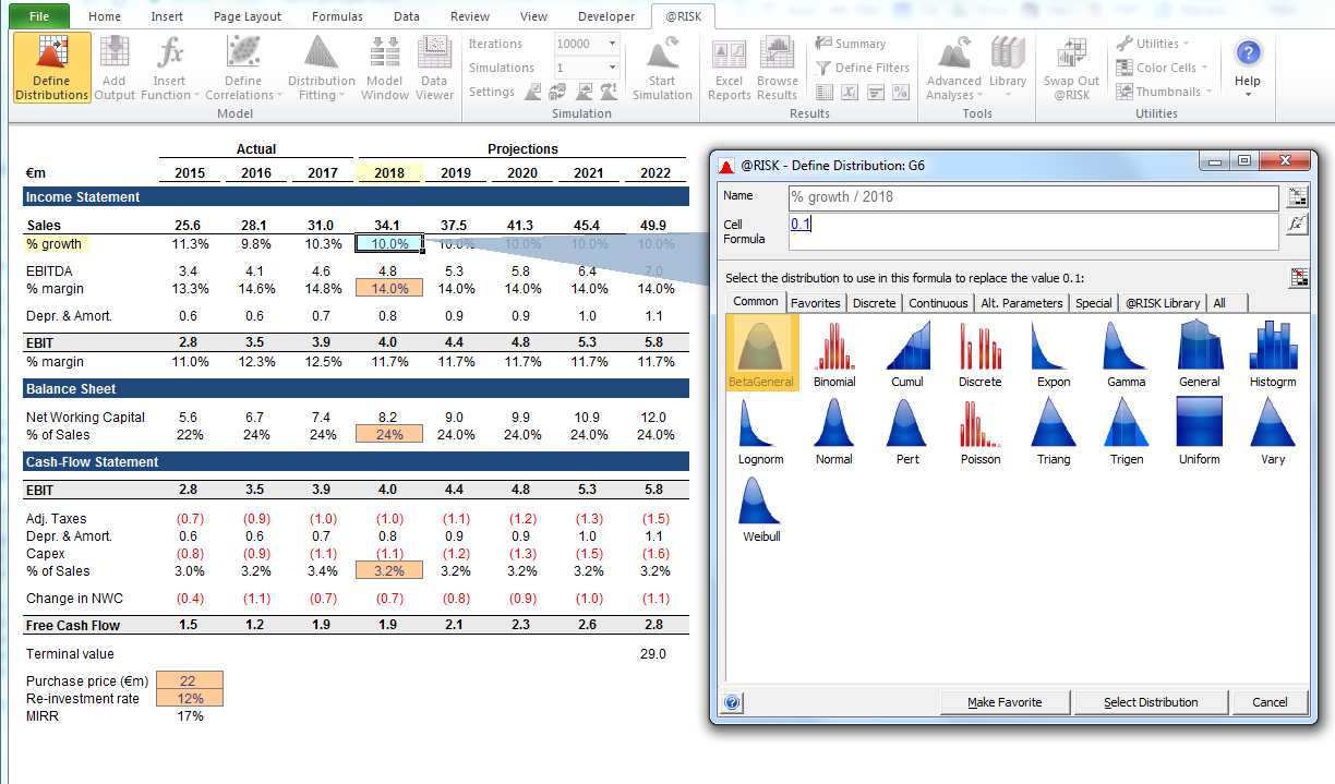
You then select one from the palette of distributions that comes up. The @RISK software offers more than 70 different distributions to choose from, so choosing one can seem overwhelming at first. Below is a guide to a handful I use most often:
|
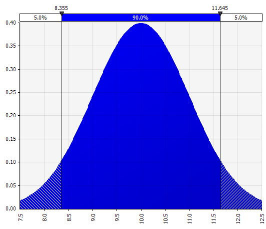
Normal. Defined by mean and standard deviation. This is a good starting point due to its simplicity, and suitable as an extension to the Morningstar approach, where you define a distribution that covers perhaps already defined scenarios or ranges for a given input, ensuring that the cases are symmetrical around the base case and that the probabilities in each tail look reasonable (say 25% as in the Morningstar example). |
 |
|
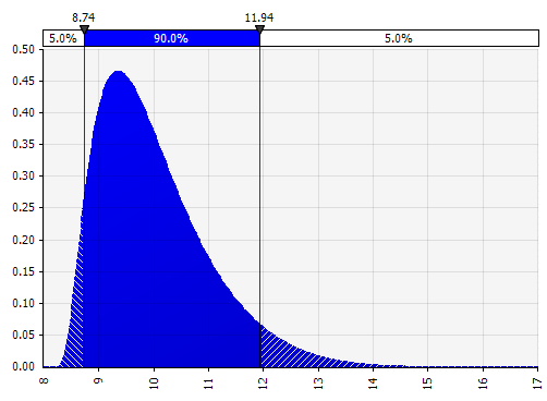
Johnson Moments. Choosing this allows you to define skewed distributions and distributions with fatter or thinner tails (technically adding skewness and kurtosis parameters). Behind the scenes, this uses an algorithm to choose one of four distributions which reflects the four chosen parameters, but that is invisible to the user---all we have to focus on are the parameters.
|
 |
|
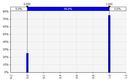
Discrete. Where probabilities are given to two or more specific values. Returning to the staged R&D project example in the beginning, the probability of success at each stage is modeled as a binary discrete distribution, with an outcome of 1 representing success and 0 failure. |
 |
|
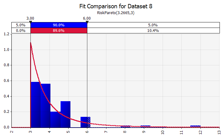
Distribution Fitting. When you have a large amount of historical data points, the distribution fitting functionality is useful. This does not mean three or four years of historical sales growth, for example, but time series data such as commodities prices, currency exchange rates, or other market prices where history can give useful information about future trends and the degree of uncertainty. |
 |
|
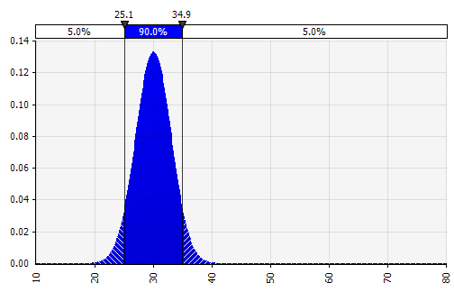
Combining several different distributions into one. To mitigate the potential impact of individual biases, it is often a good idea to incorporate the input of different sources into an assumption, and/or to review and discuss the findings. There are different approaches:
|
 Weight: 20% 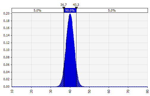 Weight: 20% 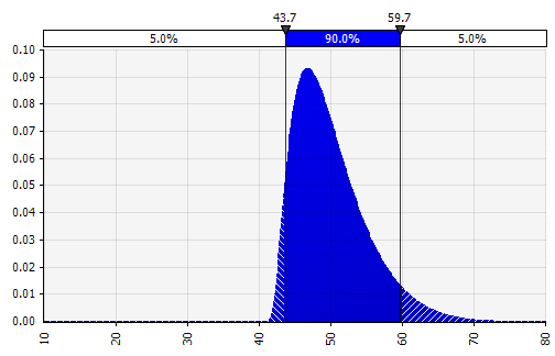 Weight: 60% 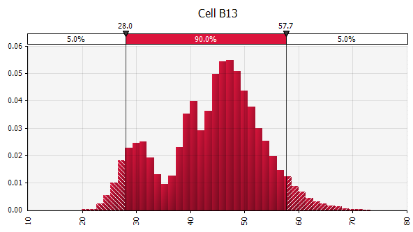 |
|
Freehand. To quickly illustrate a distribution as part of discussions or if you need a distribution when drafting a model not easily created from the existing palette, the freehand functionality is useful. As the name implies, this allows you to draw the distribution using a simple painting tool. |
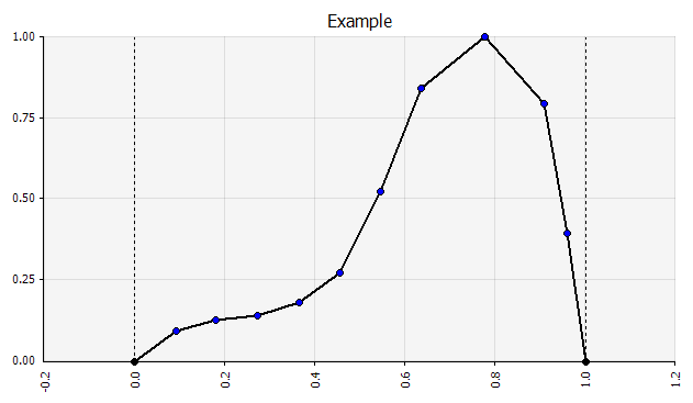 |
Now we see a visualization of the distribution, with a few parameters on the left-hand side. The mean and standard deviation symbols should look familiar. In the case of a normal distribution, the mean would be what we previously entered as a single value in the cell. Here is the 2018 sales probability distribution as an example, with 10% representing the mean. Whereas your typical model would either focus only on the 10% figure, or have “bull” and “bear” scenarios with perhaps 15% and 5% growth respectively, this now provides information about the full range of expected potential outcomes.
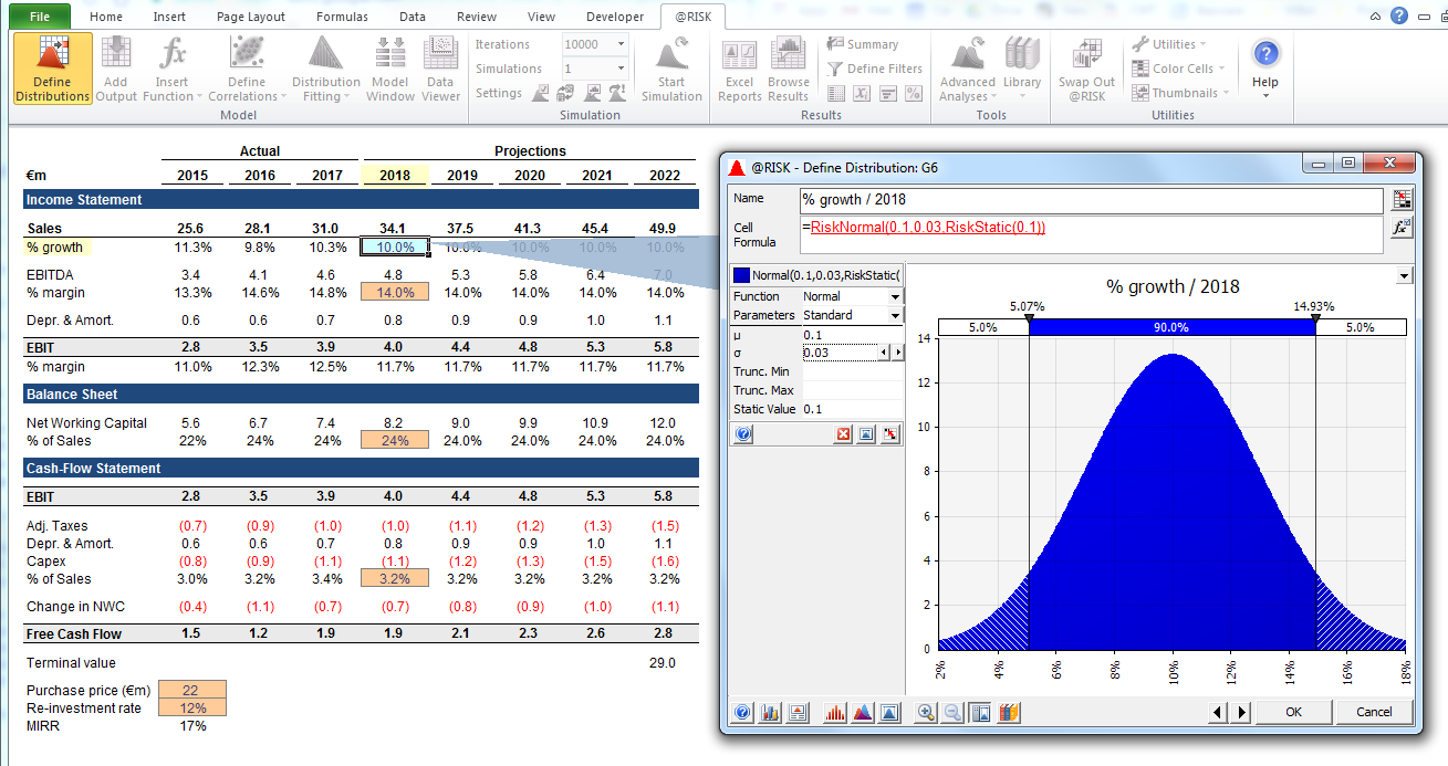
One benefit of Monte Carlo simulations is that low-probability tail outcomes can trigger thinking and discussions. Only displaying upside and downside scenarios can introduce the risk that decision-makers interpret those as the outer bounds, dismissing any scenarios that lie outside. This can result in flawed decision-making, with exposure to outcomes that lie beyond the organization’s or individual’s tolerance for risk. Even a 5% or 1% probability may be unacceptable if the scenario in question would have catastrophic consequences.
Step 3. Expanding the Revenue Forecast from One Year to Several
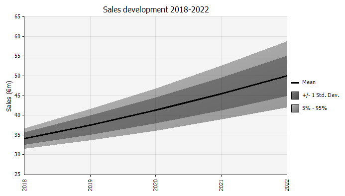
With Monte Carlo modeling, be mindful of how uncertainty and probability distributions stack on top of each other, such as over time. Let’s review an example. Since sales in each year depends on growth in the preceding ones, we can visualize and see that our estimate of 2022 sales is more uncertain than that for 2018 (shown using the standard deviations and 95% confidence intervals in each year). For the sake of simplicity, the below example specifies the growth for one year, 2018, and then applies that same growth rate to each of the following years until 2022. Another approach is to have five independent distributions, one for each year.

Step 4. Continuing down the Income Statement—Expressing Margins as Probability Distributions
We now estimate a probability distribution for the EBIT margin in 2018 (highlighted below) similarly to how we did it for sales growth.
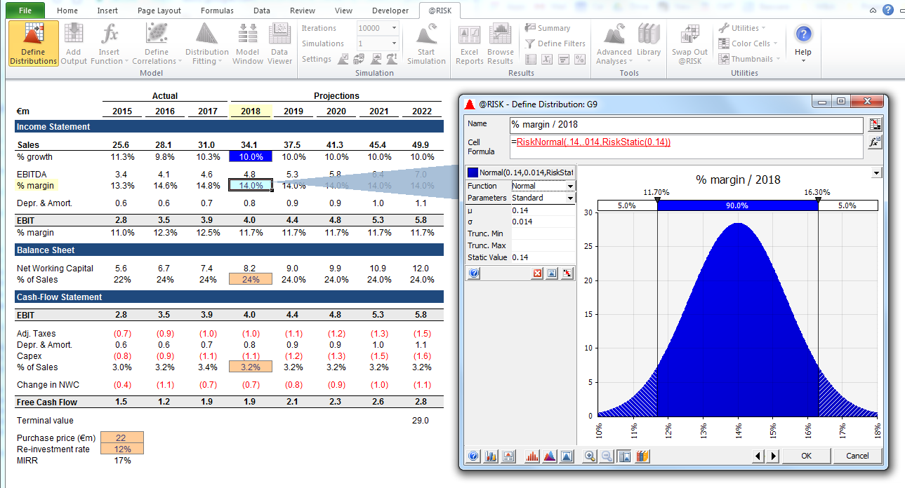
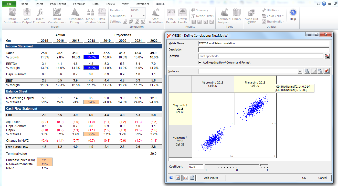
Here, we can use the correlation function to simulate a situation where there is a clear correlation between relative market share and profitability, reflecting economies of scale. Scenarios with higher sales growth relative to the market and correspondingly higher relative market share can be modeled to have a positive correlation with higher EBIT margins. In industries where a firm’s fortune is strongly correlated with some other external factor, such as oil prices or foreign exchange rates, defining a distribution for that factor and modeling a correlation with sales and profitability can make sense.
Depending on the time available, size of transaction, and other factors, it often makes sense to build an operating model and input the most uncertain variables explicitly. These include: product volumes and prices, commodity prices, FX rates, key overhead line items, monthly active users, and average revenue per unit (ARPU). It’s also possible to model beyond amount variables such as development time, time to market, or market adoption rate.
Step 5. Balance Sheet and Cash-flow Statement
Using the outlined approach, we can now continue through the balance sheet and cash flow statement, populating with assumptions and using probability distributions where it makes sense.
A note on capex: this can be modeled either in absolute amounts or as a percentage of sales, potentially in combination with larger stepwise investments; a manufacturing facility may for example have a clear capacity limit and a large expansion investment or a new facility necessary when sales exceed the threshold. Since each of the say 1,000 or 10,000 iterations will be a complete recalculation of the model, a simple formula that triggers the investment cost if/when a certain volume is reached can be used.
Step 6. Finalizing the Model
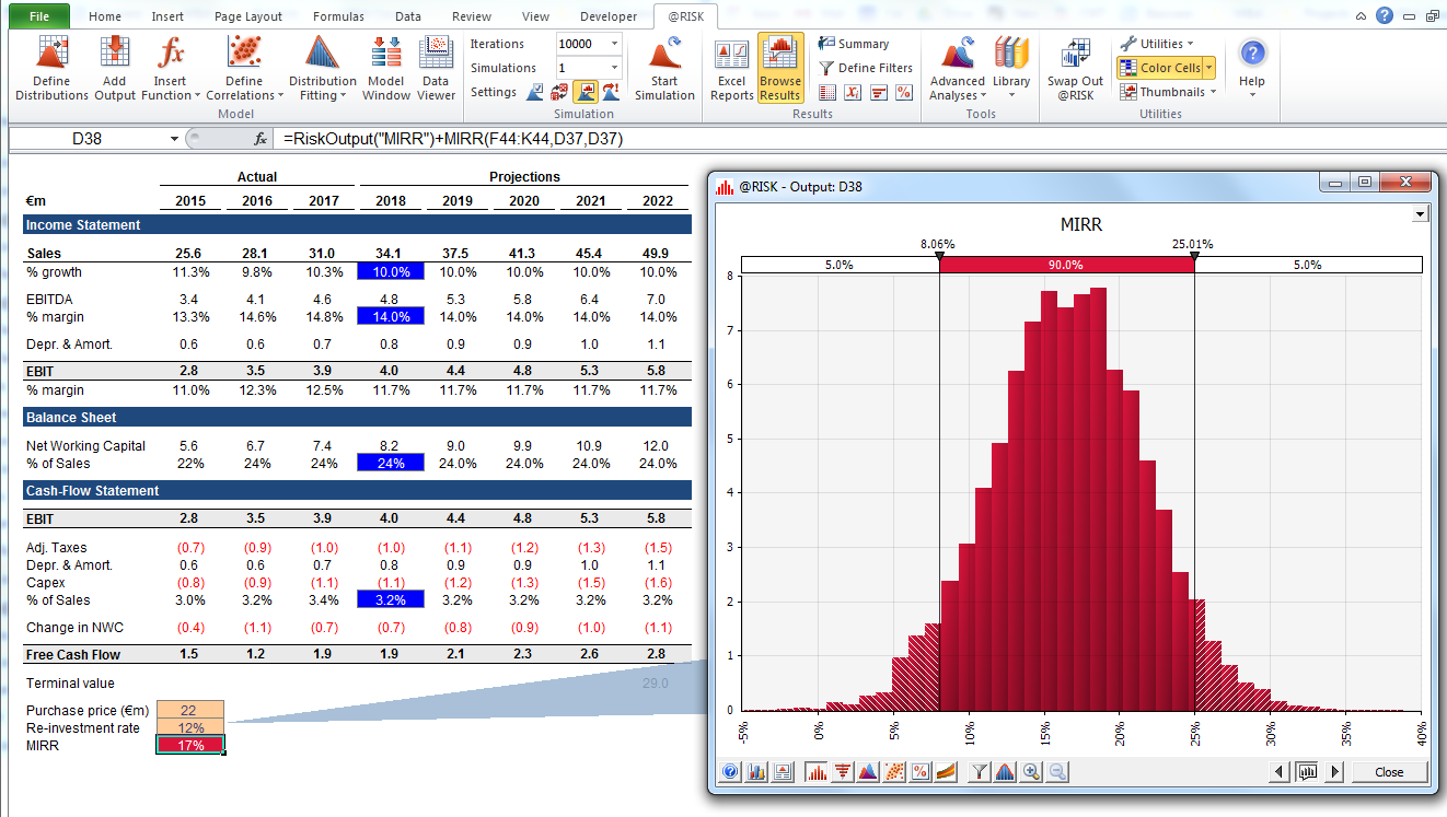
Building a Monte Carlo model has one additional step compared to a standard financial model: The cells where we want to evaluate the results need to be specifically designated as output cells. The software will save the results of each iteration of the simulation for those cells for us to evaluate after the simulation is finished. All cells in the entire model are recalculated with each iteration, but the results of the iterations in other cells, which are not designated as input or output cells, are lost and cannot be analyzed after the simulation finishes. As you can see in the screenshot below, we designate the MIRR result cell to be an output cell.
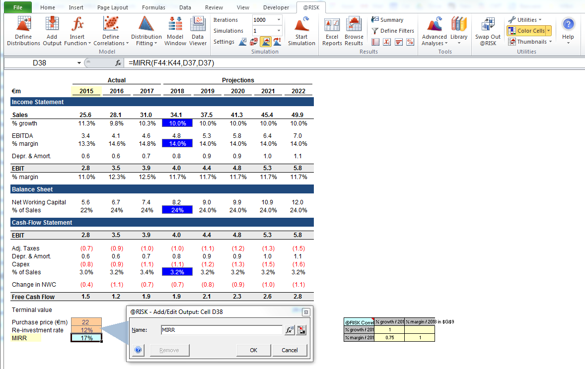
Once you have finished building the model, it is time to run the simulation for the first time by simply pressing “start simulation” and waiting for a few seconds.
Step 7. Interpreting the Results
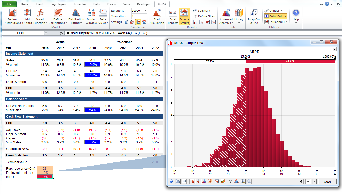
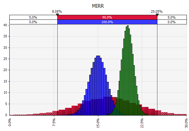
Outputs Expressed as Probabilities. Whereas our model previously gave us a single value for the modified IRR, we can now clearly see that there are a number of potential outcomes around that value, with different probabilities. This allows us to rephrase questions, such as “Will we hit our hurdle return rate with this investment?” to “How likely are we to hit or exceed our hurdle rate?” You can explore which outcomes are most likely using, for example, a confidence interval. The visualization is helpful when communicating the results to different stakeholders, and you can overlay outputs from other transactions to visually compare how attractive and (un)certain the current one is compared to others (see below).
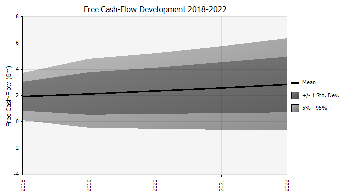
Understanding the degree of uncertainty in the final result. If we generate a chart of cash-flow variability over time, similar to what we did initially for sales, it becomes clear that the variability in free cash flow becomes significant even with relatively modest uncertainty in sales and the other inputs we modeled as probability distributions, with results ranging from around €0.5 million to €5.0 million—a factor of 10x—even just one standard deviation from the mean. This is the result of stacking uncertain assumptions on top of each other, an effect that compounds both “vertically” over the years, and “horizontally” down through the financial statements. The visualizations provide information about both types of uncertainty.
Sensitivity analysis: Introducing the tornado graph. Another important area is to understand which inputs have the greatest impact on your final result. A classical example is how the importance of discount rate or terminal value assumptions is often given too little weight relative to cash flow forecasting. One common way to handle this is by using matrices where you put one key input on each axis and then calculate the result in each cell (see below). This is useful especially in situations where decisions hinge on one or a few key assumptions—in these “what you have to be believe” situations, decision-makers on (for example) an investment committee or a senior management team may have different views of those key assumptions, and a matrix such as the one above allows each one of them to find a result value corresponding to their view, and can decide, vote, or give advice based on that.

Enhancing with Monte Carlo simulations. When using Monte Carlo simulations, that approach can be complemented with another: the tornado diagram. This visualization lists the different uncertain inputs and assumptions on the vertical axis and then shows how large the impact of each is on the end result.
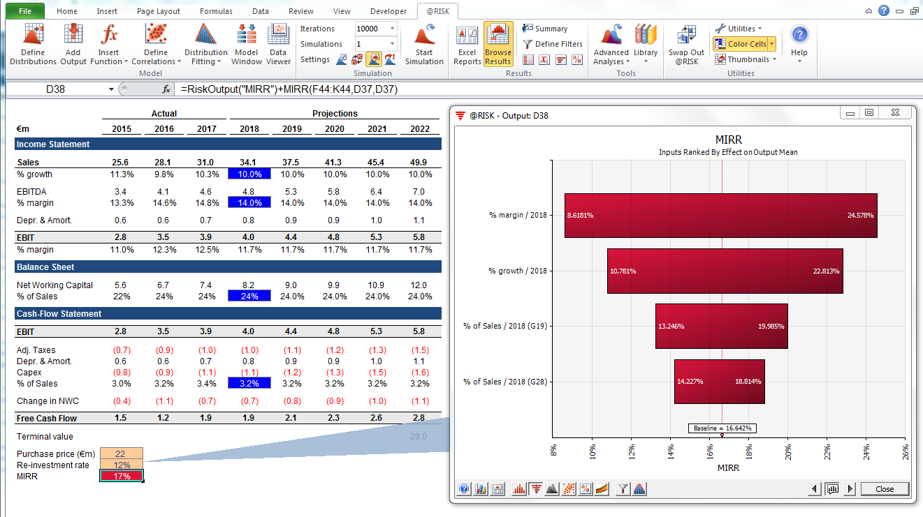
This has several uses, one of which is that it allows those preparing the analysis to ensure that they are spending time and effort on understanding and validating the assumptions roughly corresponding to how important each is for the end result. It can also guide the creation of a sensitivity analysis matrix by highlighting which assumptions really are key.
Another potential use case is to allocate engineering hours, funds, or other scarce resources to validating and narrowing the probability distributions of the most important assumptions. An example of this in practice was a VC-backed cleantech startup where I used this method to support decision-making both to allocate resources and to validate the commercial viability of its technology and business model, making sure you solve the most important problems, and gather the most important information first. Update the model, move the mean values, and adjust the probability distributions, and continually reassess if you are focused on solving the right problems.
A Few Words of Caution: Different Types of Uncertainty
Probability is not a mere computation of odds on the dice or more complicated variants; it is the acceptance of the lack of certainty in our knowledge and the development of methods for dealing with our ignorance. – Nassim Nicholas Taleb
It is useful to distinguish between risk, defined as situations with future outcomes that are unknown but where we can calculate their probabilities (think roulette), and uncertainty, where we cannot estimate the probabilities of events with any degree of certainty.
In business and finance, most situations facing us in practice will lie somewhere in between those two. The closer we are to the risk end of that spectrum, the more confident we can be that when using probability distributions to model possible future outcomes, as we do in Monte Carlo simulations, those will accurately capture the situation facing us.
The closer we get to the uncertainty end of the spectrum, the more challenging or even dangerous it can be to use Monte Carlo simulations (or any quantitative approach). The concept of “fat tails,” where a probability distribution may be useful but the one used has the wrong parameters, has received lots of attention in finance, and there are situations where even the near-term future is so uncertain that any attempt to capture it in a probability distribution at all will be more misleading than helpful.
In addition to keeping the above in mind, is also important to 1) be mindful of the shortcomings of your models, 2) be vigilant against overconfidence, which can be amplified by more sophisticated tools, and 3) bear in mind the risk of significant events that may lie outside what has been seen before or the consensus view.
At the End of the Day, It’s about the Mindset, Not the Technical Solution
There are two concepts here and it is important to separate them: one is the recognition of uncertainty and the mindset of thinking in probabilities, and the other is one practical tool to support that thinking and have constructive conversations about it: Monte Carlo simulations in spreadsheets.
I don’t use Monte Carlo simulations in all models I build or work on today, or even a majority. But the work I have done with it influences how I think about forecasting and modeling. Just doing this type of exercise a few times, or even once, can influence how you view and make decisions. As with any model we use, this method remains a gross simplification of a complex world, and forecasters in economics, business, and finance have a disappointing track record when evaluated objectively.
Our models are far from perfect but, over years and decades, and millions or billions of dollars/euros invested or otherwise allocated, even a small improvement in your decision-making mindset and processes can add significant value.
I spend 98% of my time on 2% probabilities – Lloyd Blankfein
Understanding the basics
What is a Monte Carlo simulation used for?
Monte Carlo simulations use probability distributions to model and visualize a forecast’s full range of possible outcomes. This can be done on an aggregate level and for individual inputs, assumptions, and drivers. Monte Carlo methods are then used to calculate the probability distributions at an aggregate level.
Why do they call it the Monte Carlo simulation?
Monte Carlo simulations earn their name from the area of Monte Carlo in Monaco, which is world-famous for its high-end casinos. Random outcomes are central to the technique, just as they are to roulette and slot machines.
Stefan Thelin
Lund, Sweden
Member since September 20, 2017
About the author
Stefan is the Director of Data-Driven Insights and Analytics for Cargotec, a leading provider of cargo and loading solutions. He has also served as an M&A director and a startup CFO, and led financial modeling and analysis as a leveraged finance manager at the Royal Bank of Scotland.
Expertise
PREVIOUSLY AT


