A Deep Dive Into Reinforcement Learning
Machine learning and artificial intelligence are popular topics, vast domains with multiple paradigms to solve any given challenge.
In this article, Toptal Machine Learning Expert Adam Stelmaszczyk walks us through implementing deep Q-learning, a fundamental algorithm in the AI/ML world, with modern libraries such as TensorFlow, TensorBoard, Keras, and OpenAI Gym.
A PhD candidate specializing in AI and one of Europe’s top tech entrepreneurs, Adam is a team player and active F/OSS contributor.
PREVIOUSLY AT

Let’s take a deep dive into reinforcement learning. In this article, we will tackle a concrete problem with modern libraries such as TensorFlow, TensorBoard, Keras, and OpenAI gym. You will see how to implement one of the fundamental algorithms called deep $Q$-learning to learn its inner workings. Regarding the hardware, the whole code will work on a typical PC and use all found CPU cores (this is handled out of the box by TensorFlow).
The problem is called Mountain Car: A car is on a one-dimensional track, positioned between two mountains. The goal is to drive up the mountain on the right (reaching the flag). However, the car’s engine is not strong enough to climb the mountain in a single pass. Therefore, the only way to succeed is to drive back and forth to build up momentum.
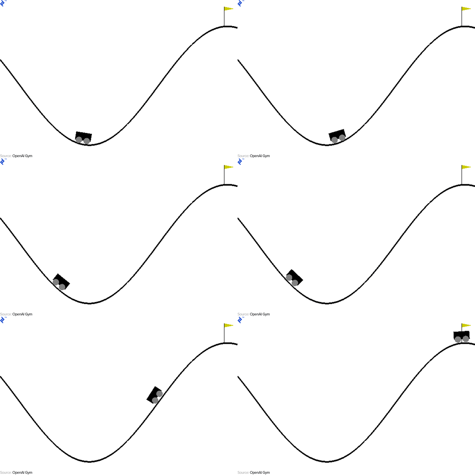
This problem was chosen because it is simple enough to find a solution with reinforcement learning in minutes on a single CPU core. However, it is complex enough to be a good representative.
First, I will give a brief summary of what reinforcement learning does in general. Then, we will cover basic terms and express our problem with them. After that, I will describe the deep $Q$-learning algorithm and we will implement it to solve the problem.
Reinforcement Learning Basics
Reinforcement learning in the simplest words is learning by trial and error. The main character is called an “agent,” which would be a car in our problem. The agent makes an action in an environment and is given back a new observation and a reward for that action. Actions leading to bigger rewards are reinforced, hence the name. As with many other things in computer science, this one was also inspired by observing live creatures.
The agent’s interactions with an environment are summarized in the following graph:
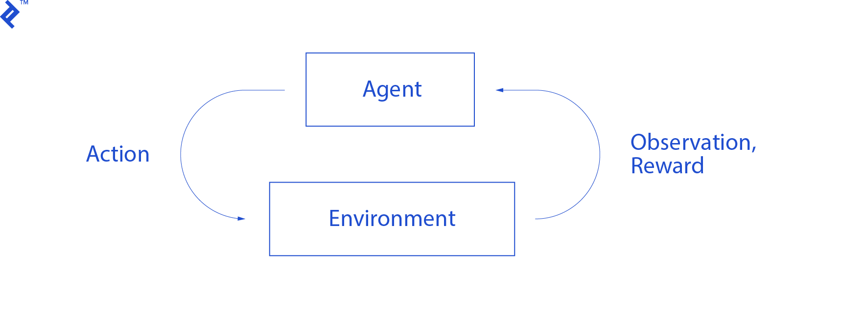
The agent gets an observation and reward for the performed action. Then it makes another action and takes step two. The environment now returns a (probably) slightly different observation and reward. This continues until the terminal state is reached, signaled by sending “done” to an agent. The whole sequence of observations > actions > next_observations > rewards is called an episode (or trajectory).
Going back to our Mountain Car: our car is an agent. The environment is a black-box world of one-dimensional mountains. The car’s action boils down to only one number: if positive, the engine pushes the car to the right. If negative, it pushes the car to the left. The agent perceives an environment through an observation: the car’s X position and velocity. If we want our car to drive on top of the mountain, we define the reward in a convenient way: The agent gets -1 to its reward for every step in which it hasn’t reached the goal. When it reaches the goal, the episode ends. So, in fact, the agent is punished for not being in a position we want it to be. The faster he reaches it, the better for him. The agent’s goal is to maximize the total reward, which is the sum of rewards from one episode. So if it reaches the desired point after, e.g., 110 steps, it receives a total return of -110, which would be a great result for Mountain Car, because if it doesn’t reach the goal, then it is punished for 200 steps (hence, a return of -200).
This is the whole problem formulation. Now, we can give it to the algorithms, which are already powerful enough to solve such problems in a matter of minutes (if well tuned). It’s worth noting that we don’t tell the agent how to achieve the goal. We don’t even provide any hints (heuristics). The agent will find a way (a policy) to win on its own.
Setting Up The Environment
First, copy the whole tutorial code onto your disk:
git clone https://github.com/AdamStelmaszczyk/rl-tutorial
cd rl-tutorial
Now, we need to install Python packages that we will use. To not install them in your userspace (and risk collisions), we will make it clean and install them in the conda environment. If you do not have conda installed, please follow https://conda.io/docs/user-guide/install/index.html.
To create our conda environment:
conda create -n tutorial python=3.6.5 -y
To activate it:
source activate tutorial
You should see (tutorial) near your prompt in the shell. It means that a conda environment with the name “tutorial” is active. From now on, all the commands should be executed within that conda environment.
Now, we can install all dependencies in our hermetic conda environment:
pip install -r requirements.txt
We are done with the installation, so let’s run some code. We don’t need to implement the Mountain Car environment ourselves; the OpenAI Gym library provides that implementation. Let’s see a random agent (an agent that takes random actions) in our environment:
import gym

env = gym.make('MountainCar-v0')
done = True
episode = 0
episode_return = 0.0
for episode in range(5):
   for step in range(200):
       if done:
           if episode > 0:
               print("Episode return: ", episode_return)
           obs = env.reset()
           episode += 1
           episode_return = 0.0
           env.render()
       else:
           obs = next_obs
       action = env.action_space.sample()
       next_obs, reward, done, _ = env.step(action)
       episode_return += reward
       env.render()
This is see.py file; to run it, execute:
python see.py
You should see a car going randomly back and forth. Each episode will consist of 200 steps; the total return will be -200.

Now we need to replace random actions with something better. There are many algorithms one could use. For an introductory tutorial, I think an approach called deep $Q$-learning is a good fit. Understanding that method gives a firm foundation for learning other approaches.
Deep $Q$-learning
The algorithm that we will use was first described in 2013 by Mnih et al. in Playing Atari with Deep Reinforcement Learning and polished two years later in Human-level control through deep reinforcement learning. Many other works are built upon those results, including the current state-of-the-art algorithm Rainbow (2017):
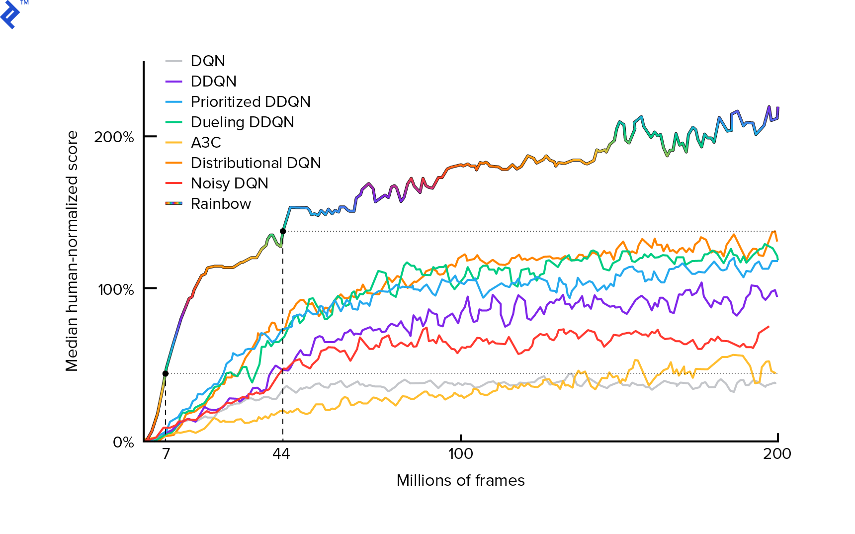
Rainbow achieves superhuman performance on many Atari 2600 games. We will focus on the basic DQN version, with as small a number of additional improvements as possible, to keep this tutorial to a reasonable size.
A policy, typically denoted $π(s)$, is a function returning probabilities of taking individual actions in a given state $s$. So, for example, a random Mountain Car policy returns for any state: 50% left, 50% right. During gameplay, we sample from that policy (distribution) to obtain real actions.
$Q$-learning (Q is for Quality) refers to the action-value function denoted $Q_π(s, a)$. It returns the total return from a given state $s$, choosing action $a$, following a concrete policy $π$. The total return is the sum of all rewards in one episode (trajectory).
If we knew the optimal $Q$-function, denoted $Q^*$, we could solve the game easily. We would just follow the actions with the highest value of $Q^*$, i.e., the highest expected return. This guarantees that we will reach the highest possible return.
However, we often don’t know $Q^*$. In such cases, we can approximate—or “learn”—it from the interactions with the environment. This is the “$Q$-learning” part in the name. There’s also the word “deep” in it because, to approximate that function, we will use deep neural networks, which are universal function approximators. Deep neural networks that approximate $Q$-values were named Deep Q-Networks (DQN). In simple environments (with the number of states fitting in memory), one could just use a table instead of a neural net to represent the $Q$-function, in which instance it would be named “tabular $Q$-learning.”
So our goal now is to approximate the $Q^*$ function. We will use the Bellman equation:
\[Q(s, a) = r + γ \space \textrm{max}_{a'} Q(s', a')\]$s’$ is the state after $s$. $γ$ (gamma), typically 0.99, is a discount factor (it’s a hyperparameter). It places a smaller weight on future rewards (because they are less certain than immediate rewards with our imperfect $Q$). The Bellman equation is central to deep $Q$-learning. It says that the $Q$-value for a given state and action is a reward $r$ received after taking action $a$ plus the highest $Q$-value for the state we land in $s’$. The highest is in a sense that we are choosing an action $a’$, which leads to the highest total return from $s’$.
With the Bellman equation, we can use supervised learning to approximate $Q^*$. The $Q$-function will be represented (parametrized) by neural network weights denoted as $θ$ (theta). A straightforward implementation would take a state and an action as the network input and output the Q-value. The inefficiency is that if we want to know $Q$-values for all the actions in a given state, we need to call $Q$ as many times as there are actions. There is a much better way: to take only the state as an input and output $Q$-values for all possible actions. Thanks to that, we can get $Q$-values for all the actions in just one forward pass.
We start training the $Q$ network with random weights. From the environment, we obtain many transitions (or “experiences”). These are tuples of (state, action, next state, reward) or, in short, ($s$, $a$, $s’$, $r$). We store thousands of them in a ring buffer called “experience replay.” Then, we sample experiences from that buffer with the desire that the Bellman equation will hold for them. We could have skipped the buffer and applied experiences one by one (this is called “online” or “on-policy”); the problem is that subsequent experiences are highly correlated with each other and DQN trains poorly when this occurs. That’s why the experience replay was introduced (an “offline,” “off-policy” approach) to break out this data correlation. The code of our simplest ring buffer implementation can be found in the replay_buffer.py file, I encourage you to read it.
In the beginning, since our neural network weights were random, the left-hand side value of the Bellman equation will be far from the right-hand side. The squared difference will be our loss function. We will minimize the loss function by changing the neural network weights $θ$. Let’s write down our loss function:
\[L(θ) = [Q(s, a) - r - γ \space \textrm{max}_{a'}Q(s', a')]^2\]It’s a rewritten Bellman equation. Let’s say we sampled an experience ($s$, left, $s’$, -1) from the Mountain Car experience replay. We do a forward pass through our $Q$ network with state $s$ and for action left it gives us -120, for example. So, $Q(s, \textrm{left}) = -120$. Then we feed $s’$ to the network, which gives us, e.g., -130 for left and -122 for right. So clearly the best action for $s’$ is right, thus $\textrm{max}_{a’}Q(s’, a’) = -122$. We know $r$, this is the real reward, which was -1. So our $Q$-network prediction was slightly wrong, because $L(θ) = [-120 - 1 + 0.99 ⋅ 122]^2 = (-0.22^2) = 0.0484$. So we backward propagate the error and correct the weights $θ$ slightly. If we were to calculate the loss again for the same experience, it would now be lower.
One important observation before we go to code. Let’s notice that, to update our DQN, we will do two forward passes on DQN… itself. This often leads to unstable learning. To alleviate that, for the next state $Q$ prediction, we don’t use the same DQN. We use an older version of it, which in the code is called target_model (instead of model, being the main DQN). Thanks to that, we have a stable target. We update target_model by setting it to model weights every 1000 steps. But model updates every step.
Let’s look at the code creating the DQN model:
def create_model(env):
   n_actions = env.action_space.n
   obs_shape = env.observation_space.shape
   observations_input = keras.layers.Input(obs_shape, name='observations_input')
   action_mask = keras.layers.Input((n_actions,), name='action_mask')
   hidden = keras.layers.Dense(32, activation='relu')(observations_input)
   hidden_2 = keras.layers.Dense(32, activation='relu')(hidden)
   output = keras.layers.Dense(n_actions)(hidden_2)
   filtered_output = keras.layers.multiply([output, action_mask])
   model = keras.models.Model([observations_input, action_mask], filtered_output)
   optimizer = keras.optimizers.Adam(lr=LEARNING_RATE, clipnorm=1.0)
   model.compile(optimizer, loss='mean_squared_error')
   return model
First, the function takes the dimensions of action and observation space from the given OpenAI Gym environment. It is necessary to know, for example, how many outputs our network will have. It must be equal to the number of actions. Actions are one hot encoded:
def one_hot_encode(n, action):
   one_hot = np.zeros(n)
   one_hot[int(action)] = 1
   return one_hot
So (e.g.) left will be [1, 0] and right will be [0, 1].
We can see the observations are passed as input. We also pass action_mask as a second input. Why? When calculating $Q(s,a)$, we need to know the $Q$-value only for one given action, not all of them. action_mask contains 1 for the actions that we want to pass to the DQN output. If action_mask has 0 for some action, then the corresponding $Q$-value will be zeroed on the output. The filtered_output layer is doing that. If we want all the $Q$-values (for max calculation), we can just pass all ones.
The code uses keras.layers.Dense to define a fully connected layer. Keras is a Python library for higher-level abstraction on top of TensorFlow. Under the hood, Keras creates a TensorFlow graph, with biases, proper weight initialization, and other low-level things. We could have just used raw TensorFlow to define the graph, but it won’t be a one-liner.
So observations are passed to the first hidden layer, with ReLU (rectified linear unit) activations. ReLU(x) is just a $\textrm{max}(0, x)$ function. That layer is fully connected with a second identical one, hidden_2. The output layer brings down the number of neurons to the number of actions. In the end, we have filtered_output, which just multiplies the output with action_mask.
To find $θ$ weights, we will use an optimizer named “Adam” with a mean squared error loss.
Having a model, we can use it to predict $Q$ values for given state observations:
def predict(env, model, observations):
   action_mask = np.ones((len(observations), env.action_space.n))
   return model.predict(x=[observations, action_mask])
We want $Q$-values for all the actions, thus action_mask is a vector of ones.
To do the actual training, we will use fit_batch():
def fit_batch(env, model, target_model, batch):
   observations, actions, rewards, next_observations, dones = batch
   # Predict the Q values of the next states. Passing ones as the action mask.
   next_q_values = predict(env, target_model, next_observations)
   # The Q values of terminal states is 0 by definition.
   next_q_values[dones] = 0.0
   # The Q values of each start state is the reward + gamma * the max next state Q value
   q_values = rewards + DISCOUNT_FACTOR_GAMMA * np.max(next_q_values, axis=1)
   one_hot_actions = np.array([one_hot_encode(env.action_space.n, action) for action in actions])
   history = model.fit(
       x=[observations, one_hot_actions],
       y=one_hot_actions * q_values[:, None],
       batch_size=BATCH_SIZE,
       verbose=0,
   )
   return history.history['loss'][0]
Batch contains BATCH_SIZE experiences. next_q_values is $Q(s, a)$. q_values is $r + γ \space \textrm{max}_{a’}Q(s’, a’)$ from the Bellman equation. Actions we took are one hot encoded and passed as action_mask to the input when calling model.fit(). $y$ is a common letter for a “target” in supervised learning. Here we are passing the q_values. I do q_values[:. None] to increase the array dimension because it must correspond to the dimension of one_hot_actions array. This is called slice notation if you would like to read more about it.
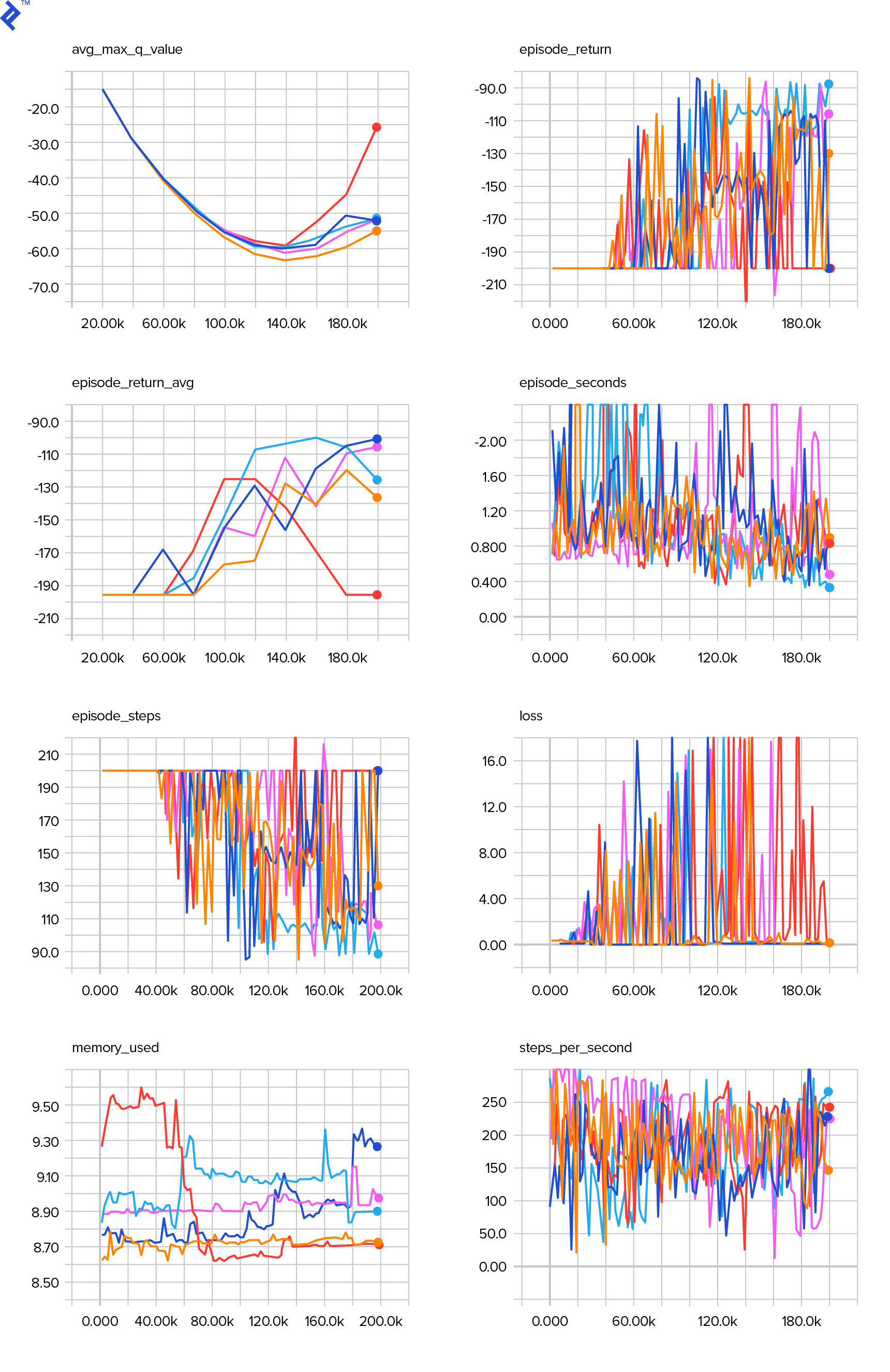
We return the loss to save it in the TensorBoard log file and later visualize. There are many other things we will monitor: how many steps per second we make, total RAM usage, what is the average episode return, etc. Let’s see those plots.
Running
To visualize the TensorBoard log file, we first need to have one. So let’s just run the training:
python run.py
This will first print the summary of our model. Then it will create a log directory with the current date and start the training. Every 2000 steps, a logline will be printed similar to this:
episode 10 steps 200/2001 loss 0.3346639 return -200.0 in 1.02s 195.7 steps/s 9.0/15.6 GB RAM
Every 20,000, we will evaluate our model on 10,000 steps:
Evaluation
100%|█████████████████████████████████████████████████████████████████████████████████| 10000/10000 [00:07<00:00, 1254.40it/s]
episode 677 step 120000 episode_return_avg -136.750 avg_max_q_value -56.004
After 677 episodes and 120,000 steps, the average episode return improved from -200 to -136.75! It’s definitely learning. What avg_max_q_value is I’m leaving as a good exercise to the reader. But it’s a very useful statistic to look at during training.
After 200,000 steps, our training is done. On my four-core CPU, it takes about 20 minutes. We can look inside the date-log directory, e.g., 06-07-18-39-log. There will be four model files with the .h5 extension. This is a snapshot of TensorFlow graph weights, we save them every 50,000 steps to later have a look at the policy we learned. To view it:
python run.py --model 06-08-18-42-log/06-08-18-42-200000.h5 --view
To see the other possible flags: python run.py --help.
Now, the car is doing a much better job of reaching the desired goal. In the date-log directory, there is also the events.out.* file. This is the file where TensorBoard stores its data. We write to it using the simplest TensorBoardLogger defined in loggers.py. To view the events file, we need to run the local TensorBoard server:
tensorboard --logdir=.
--logdir just points to the directory in which there are date-log directories, in our case, this will be the current directory, so .. TensorBoard prints the URL at which it is listening. If you open up http://127.0.0.1:6006, you should see eight plots similar to these:
Wrapping Up
train() does all the training. We first create the model and replay the buffer. Then, in a loop very similar to the one from see.py, we interact with the environment and store experiences in the buffer. What’s important is that we follow an epsilon-greedy policy. We could always choose the best action according to the $Q$-function; however, that discourages exploration, which harms overall performance. So to enforce exploration with epsilon probability, we perform random actions:
def greedy_action(env, model, observation):
   next_q_values = predict(env, model, observations=[observation])
   return np.argmax(next_q_values)


def epsilon_greedy_action(env, model, observation, epsilon):
   if random.random() < epsilon:
       action = env.action_space.sample()
   else:
       action = greedy_action(env, model, observation)
   return action
Epsilon was set to 1%. After 2000 experiences, the replay fills up enough to start the training. We do it by calling fit_batch() with a random batch of experiences sampled from the replay buffer:
batch = replay.sample(BATCH_SIZE)
loss = fit_batch(env, model, target_model, batch)
Every 20,000 steps, we evaluate and log the results (evaluation is with epsilon = 0, totally greedy policy):
if step >= TRAIN_START and step % EVAL_EVERY == 0:
   episode_return_avg = evaluate(env, model)
   q_values = predict(env, model, q_validation_observations)
   max_q_values = np.max(q_values, axis=1)
   avg_max_q_value = np.mean(max_q_values)
   print(
       "episode {} "
       "step {} "
       "episode_return_avg {:.3f} "
       "avg_max_q_value {:.3f}".format(
           episode,
           step,
           episode_return_avg,
           avg_max_q_value,
       ))
   logger.log_scalar('episode_return_avg', episode_return_avg, step)
   logger.log_scalar('avg_max_q_value', avg_max_q_value, step)
The whole code is about 300 lines, and run.py contains about 250 of the most important ones.
One can notice there are a lot hyperparameters:
DISCOUNT_FACTOR_GAMMA = 0.99
LEARNING_RATE = 0.001
BATCH_SIZE = 64
TARGET_UPDATE_EVERY = 1000
TRAIN_START = 2000
REPLAY_BUFFER_SIZE = 50000
MAX_STEPS = 200000
LOG_EVERY = 2000
SNAPSHOT_EVERY = 50000
EVAL_EVERY = 20000
EVAL_STEPS = 10000
EVAL_EPSILON = 0
TRAIN_EPSILON = 0.01
Q_VALIDATION_SIZE = 10000
And that’s even not all of them. There is also a network architecture—we used two hidden layers with 32 neurons, ReLU activations, and Adam optimizer, but there are lots of other options. Even small changes can have a huge impact on training. A lot of time can be spent tuning hyperparameters. In a recent OpenAI competition, a second-place contestant found out it is possible to almost double Rainbow’s score after hyperparameter tuning. Naturally, one has to remember that it’s easy to overfit. Currently, reinforcement algorithms are struggling with knowledge transfer to similar environments. Our Mountain Car doesn’t generalize to all types of mountains right now. You can actually modify the OpenAI Gym environment and see how far the agent can generalize.
Another exercise will be to find a better set of hyperparameters than mine. It’s definitely possible. However, one training run will be not enough to judge whether your change is an improvement. There usually is a be a big difference between training runs; the variance is big. You would need many runs to determine that something is better. If you would like to read more about such important topic as reproducibility, I encourage you to read Deep Reinforcement Learning that Matters. Instead of tuning by hand, we can automate this process to some extent—if we are willing to spend more computing power on the problem. A simple approach is to prepare a promising range of values for some hyperparameters and than run a grid search (checking their combinations), with trainings running in parallel. Parallelization itself is a big topic on its own as it is crucial for high performance.
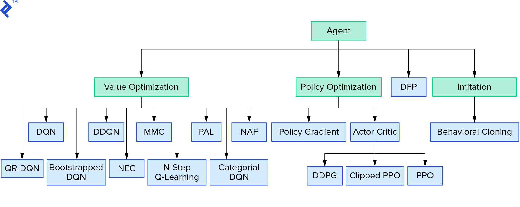
Deep $Q$-learning represents a big family of reinforcement learning algorithms that use value iteration. We tried to approximate the $Q$-function, and we just used it in a greedy manner most of the time. There is another family that uses policy iteration. They don’t focus at approximating the $Q$-function, but at finding the optimal policy $π^*$ directly. To see where value iteration fits in the landscape of reinforcement learning algorithms:
Your thoughts could be that deep reinforcement learning looks brittle. You will be right; there are many problems. You can refer to Deep Reinforcement Learning Doesn’t Work Yet and Reinforcement Learning never worked, and ‘deep’ only helped a bit.
This wraps up the tutorial. We implemented our own basic DQN for learning purposes. Very similar code can be used to achieve good performance in some of the Atari games. In practical applications, one often takes tested, high-performance implementations, e.g., one from OpenAI baselines. If you would like to see what challenges one can face when trying to apply deep reinforcement learning in a more complex environment, you can read Our NIPS 2017: Learning to Run approach. If you would like to learn more in a fun competition environment, have a look at NIPS 2018 Competitions or crowdai.org.
If you’re on your way to becoming a machine learning expert and would like to deepen your knowledge in supervised learning, check out Machine Learning Video Analysis: Identifying Fish for a fun experiment on identifying fish.
Understanding the basics
What is reinforcement learning?
Reinforcement learning is a biologically inspired trial-and-error method of training an agent. We reward the agent for good actions to reinforce the desired behavior. We also penalized bad actions, so that they happen less frequently.
What is Q in Q-learning?
Q is for “quality.” It refers to the action-value function denoted Qπ(s, a). It returns the total return from a given state s, choosing action a, following a concrete policy π. The total return is the sum of all rewards in one episode.
What is the Bellman equation?
Q(s, a) = r + γ maxa’Q(s’, a’). Verbally: Q-value for a given state and action is a reward r received after taking action a + the highest Q-value for the state we land in s’. The highest in a sense that we are choosing an action a’ that leads to the highest total return from s’.
What is Bellman's principle of optimality?
Principle of optimality: An optimal policy has the property that whatever the initial state and actions are, the remaining actions must constitute an optimal policy with regard to the state resulting from the initial action. It’s used in Q-learning, but in general in every dynamic programming technique.
What are parameters and hyperparameters?
Parameters refer to model parameters, so if using neural networks, it refers to their weights. Typically, we have thousands or millions of parameters. Hyperparameters are used to tune the learning process—e.g., learning rate, number of layers, neurons, etc. Usually, we have less than a hundred hyperparameters.
Adam Stelmaszczyk
Warsaw, Poland
Member since September 14, 2017
About the author
A PhD candidate specializing in AI and one of Europe’s top tech entrepreneurs, Adam is a team player and active F/OSS contributor.
PREVIOUSLY AT

