The Rise Of Automated Trading: Machines Trading the S&P 500
More than 60 percent of trading activities with different assets rely on automated trading and machine learning instead of human traders. Today, specialized programs based on particular algorithms and learned patterns automatically buy and sell assets in various markets, with a goal to achieve a positive return in the long run.
In this article, Toptal Freelance Data Scientist Andrea Nalon explains how to predict, using machine learning and Python, which trade should be made next on the S&P 500 to get a positive gain.
With an MCE and extensive ML and quantitative analysis training, Andrea’s a data science experience covers R, Python, VBA, Excel, and SQL.
Expertise
PREVIOUSLY AT

Nowadays, more than 60 percent of trading activities with different assets (such as stocks, index futures, commodities) are not made by “human being” traders anymore, instead relying on automated trading. There are specialized programs based on particular algorithms that automatically buy and sell assets over different markets, meant to achieve a positive return in the long run.
In this article, I’m going to show you how to predict, with good accuracy, how the next trade should be placed to get a positive gain. For this example, as the underlying asset to trade, I selected the S&P 500 index, the weighted average of 500 US companies with bigger capitalization. A very simple strategy to implement is to buy the S&P 500 index when Wall Street Exchange starts trading, at 9:30 AM, and selling it at the closing session at 4:00 PM Eastern Time. If the closing price of the index is higher than the opening price, there is a positive gain, whereas a negative gain would be achieved if the closing price is lower than the opening price. So the question is: how do we know if the trading session will end up with a closing price higher than opening price? Machine Learning is a powerful tool to achieve such a complex task, and it can be a useful tool to support us with the trading decision.
Machine Learning is the new frontier of many useful real-life applications. Financial trading is one of these, and it’s used very often in this sector. An important concept about Machine Learning is that we do not need to write code for every kind of possible rules, such as pattern recognition. This is because every model associated with Machine Learning learns from the data itself, and then can be later used to predict unseen new data.
Disclaimer: The purpose of this article is to show how to train Machine Learning methods, and in the provided code examples not every function is explained. This article is not intended to let one copy and paste all the code and run the same provided tests, as some details are missing that were out of the scope the article. Also, base knowledge of Python is required. The main intention of the article is to show an example of how machine learning may be effective to predict buys and sells in the financial sector. However, trade with real money means to have many other skills, such as money management and risk management. This article is just a small piece of the “big picture”.
Building Your First Financial Data Automated Trading Program
So, you want to create your first program to analyze financial data and predict the right trade? Let me show you how. I will be using Python for Machine Learning code, and we will be using historical data from Yahoo Finance service. As mentioned before, historical data is necessary to train the model before making our predictions.
To begin, we need to install:
- Python, and in particular I suggest using IPython notebook.
-
Yahoo Finance Python package (the exact name is
yahoo-finance) through the terminal command:pip install yahoo-finance. - A free trial version of Machine Learning package called GraphLab. Feel free to check the useful documentation of that library.
Note that only a part of GraphLab is open source, the SFrame, so to use the entire library we need a license. There is a 30 day free license and a non-commercial license for students or those one participating in Kaggle competitions. From my point of view, GraphLab Create is a very intuitive and easy to use library to analyze data and train Machine Learning models.
Digging in the Python Code
Let’s dig in with some Python code to see how to download financial data from the Internet. I suggest using IPython notebook to test the following code, because IPython has many advantages compared to a traditional IDE, especially when we need to combine source code, execution code, table data and charts together on the same document. For a brief explanation to use IPython notebook, please look at the Introduction to IPython Notebook article.
So, let’s create a new IPython notebook and write some code to download historical prices of S&P 500 index. Note, if you prefer to use other tools, you can start with a new Python project in your preferred IDE.
import graphlab as gl
from __future__ import division
from datetime import datetime
from yahoo_finance import Share

# download historical prices of S&P 500 index
today = datetime.strftime(datetime.today(), "%Y-%m-%d")
stock = Share('^GSPC') # ^GSPC is the Yahoo finance symbol to refer S&P 500 index
# we gather historical quotes from 2001-01-01 up to today
hist_quotes = stock.get_historical('2001-01-01', today)
# here is how a row looks like
hist_quotes[0]
{'Adj_Close': '2091.580078',
 'Close': '2091.580078',
 'Date': '2016-04-22',
 'High': '2094.320068',
 'Low': '2081.199951',
 'Open': '2091.48999',
 'Symbol': '%5eGSPC',
 'Volume': '3790580000'}
Here, hist_quotes is a list of dictionaries, and each dictionary object is a trading day with Open, High, Low, Close, Adj_close, Volume, Symbol and Date values. During each trading day, the price usually changes starting from the opening price Open to the closing price Close, and hitting a maximum and a minimum value High and Low. We need to read through it and create lists of each of the most relevant data. Also, data must be ordered by the most recent values at first, so we need to reverse it:
l_date = []
l_open = []
l_high = []
l_low = []
l_close = []
l_volume = []
# reverse the list
hist_quotes.reverse()
for quotes in hist_quotes:
    l_date.append(quotes['Date'])
    l_open.append(float(quotes['Open']))
    l_high.append(float(quotes['High']))
    l_low.append(float(quotes['Low']))
    l_close.append(float(quotes['Close']))
    l_volume.append(int(quotes['Volume']))
We can pack all downloaded quotes into an SFrame object, which is a highly scalable column based data frame, and it is compressed. One of the advantages is that it can also be larger than the amount of RAM because it is disk-backed. You can check the documentation to learn more about SFrame.
So, let’s store and then check the historical data:
qq = gl.SFrame({'datetime' : l_date,
          'open' : l_open,
          'high' : l_high,
          'low' : l_low,
          'close' : l_close,
          'volume' : l_volume})
# datetime is a string, so convert into datetime object
qq['datetime'] = qq['datetime'].apply(lambda x:datetime.strptime(x, '%Y-%m-%d'))

# just to check if data is sorted in ascending mode
qq.head(3)
| close | datetime | high | low | open | volume |
| 1283.27 | 2001-01-02 00:00:00 | 1320.28 | 1276.05 | 1320.28 | 1129400000 |
| 1347.56 | 2001-01-03 00:00:00 | 1347.76 | 1274.62 | 1283.27 | 1880700000 |
| 1333.34 | 2001-01-04 00:00:00 | 1350.24 | 1329.14 | 1347.56 | 2131000000 |
Now we can save data to disk with the SFrame method save, as follows:
qq.save(“SP500_daily.bin”)
# once data is saved, we can use the following instruction to retrieve it
qq = gl.SFrame(“SP500_daily.bin/”)
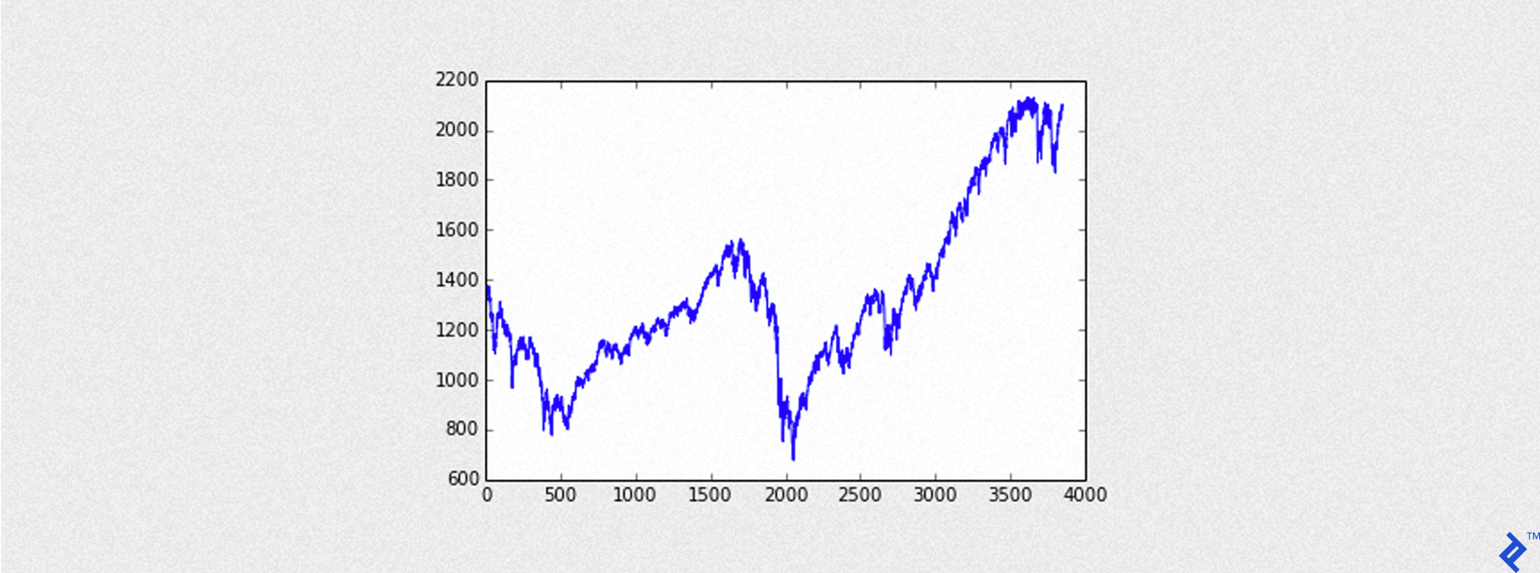
Let’s See What the S&P 500 Looks Like
To see how the loaded S&P 500 data will look like, we can use the following code:
import matplotlib.pyplot as plt
%matplotlib inline # only for those who are using IPython notebook
plt.plot(qq['close'])
The output of the code is the following graph:
Training Some Machine Learning Models
Adding Outcome
As I stated in the introductory part of this article, the goal of each model is to predict if the closing price will be higher than the opening price. Hence, in that case, we can achieve a positive return when buying the underlying asset. So, we need to add an outcome column on our data which will be the target or predicted variable. Every row of this new column will be:
-
+1for an Up day with aClosingprice higher thanOpeningprice. -
-1for a Down day with aClosingprice lower thanOpeningprice.
# add the outcome variable, 1 if the trading session was positive (close>open), 0 otherwise
qq['outcome'] = qq.apply(lambda x: 1 if x['close'] > x['open'] else -1)
# we also need to add three new columns ‘ho’ ‘lo’ and ‘gain’
# they will be useful to backtest the model, later
qq['ho'] = qq['high'] - qq['open'] # distance between Highest and Opening price
qq['lo'] = qq['low'] - qq['open'] # distance between Lowest and Opening price
qq['gain'] = qq['close'] - qq['open']
Since we need to assess some days before the last trading day, we need to lag data by one or more days. For that kind of lagging operation, we need another object from GraphLab package called TimeSeries. TimeSeries has a method shift that lags data by a certain number of rows.
ts = gl.TimeSeries(qq, index='datetime')
# add the outcome variable, 1 if the bar was positive (close>open), 0 otherwise
ts['outcome'] = ts.apply(lambda x: 1 if x['close'] > x['open'] else -1)

# GENERATE SOME LAGGED TIMESERIES
ts_1 = ts.shift(1) # by 1 day
ts_2 = ts.shift(2) # by 2 days
# ...etc....
# it's an arbitrary decision how many days of lag are needed to create a good forecaster, so
# everyone can experiment by his own decision
Adding Predictors
Predictors are a set of feature variables that must be chosen to train the model and predict our outcome. So, forecasting factor choice is crucial, if not the most important, component of the forecaster.
Just to name a few examples, a factor to consider may be if today’s close is higher than yesterday’s close, and that might be extended with two previous days’ close, etc. A similar choice can be translated with the following code:
ts['feat1'] = ts['close'] > ts_1['close']
ts['feat2'] = ts['close'] > ts_2['close']
As shown above, I’ve added two new features columns, feat1 and feat2 on our data set (ts) containing 1 if the comparison is true and 0 otherwise.
This article is intended to give an example of Machine Learning applied to the Financial sector. I prefer to focus on how Machine Learning models may be used with financial data, and we will not go into detail regarding how to choose the right factors to train the models. It is too exhaustive to explain why certain factors are used in respect to others, due to a considerable increase in complexity. My job research is to study many hypotheses of choosing factors to create a good predictor. So for a start, I suggest you experiment with lots of different combinations of factors, to see if they may increase the accuracy of the model.
# add_features is a helper function, which is out of the scope of this article,
# and it returns a tuple with:
# ts: a timeseries object with, in addition to the already included columns, also lagged columns
# as well as some features added to train the model, as shown above with feat1 and feat2 examples
# l_features: a list with all features used to train Classifier models
# l_lr_features: a list all features used to train Linear Regression models

ts, l_features, l_lr_features = add_features(ts)

# add the gain column, for trading operations with LONG only positions.
# The gain is the difference between Closing price - Opening price
ts['gain'] = ts['close'] - ts['open']

ratio = 0.8 # 80% of training set and 20% of testing set
training = ts.to_sframe()[0:round(len(ts)*ratio)]
testing = ts.to_sframe()[round(len(ts)*ratio):]
Training a Decision Tree Model
GraphLab Create has a very clean interface to implement Machine Learning models. Each model has a method create used to fit the model with a training data set. Typical parameters are:
-
training- it is a training set containing feature columns and a target column. -
target- it is the name of the column containing the target variable. -
validation_set- it is a dataset for monitoring the model’s generalization performance. In our case, we have novalidation_set. -
features- it is a list of columns names of features used for training the model. -
verbose- iftrue, print progress information during training.
Whereas other parameters are typical of the model itself, such as:
-
max_depth- it is the maximum depth of a tree.
With the following code we build our decision tree:
max_tree_depth = 6
decision_tree = gl.decision_tree_classifier.create(training, validation_set=None,
                                                   target='outcome', features=l_features,
                                                   max_depth=max_tree_depth, verbose=False)
Measuring Performance of Fitted Model
Accuracy is an important metric to evaluate the goodness of the forecaster. It is the number of correct predictions divided by the number of total data points. Since the model is fitted with training data, the accuracy evaluated with the training set is better than the one obtained with a test set.
Precision is the fraction of positive predictions that are positive. We need precision to be a number closer to 1, to achieve a “perfect” win-rate. Our decision_tree, as another classifier from GraphLab Create package, has its method evaluate to get many important metrics of the fitted model.
Recall quantifies the ability of a classifier to predict positive examples. Recall can be interpreted as the probability that a randomly selected positive example is correctly identified by the classifier. We need that precision would be a number closer to 1, to achieve a “perfect” win-rate.
The following code will show the accuracy of the fitted model both with training set and testing set:
decision_tree.evaluate(training)['accuracy'], decision_tree.evaluate(testing)['accuracy']
(0.6077348066298343, 0.577373211963589)
As shown above, the accuracy of the model with the test set is about 57 percent, which is somehow better than tossing a coin (50 percent).
Predicting Data
GraphLab Create has the same interface to predict data from different fitted models. We will use the predictmethod, which needs a test set to predict the target variable, in our case outcome. Now, we can predict data from the testing set:
predictions = decision_tree.predict(testing)
# and we add the predictions  column in testing set
testing['predictions'] = predictions

# let's see the first 10 predictions, compared to real values (outcome column)
testing[['datetime', 'outcome', 'predictions']].head(10)
| datetime | outcome | predictions |
| 2013-04-05 00:00:00 | -1 | -1 |
| 2013-04-08 00:00:00 | 1 | 1 |
| 2013-04-09 00:00:00 | 1 | 1 |
| 2013-04-10 00:00:00 | 1 | -1 |
| 2013-04-11 00:00:00 | 1 | -1 |
| 2013-04-12 00:00:00 | -1 | -1 |
| 2013-04-15 00:00:00 | -1 | 1 |
| 2013-04-16 00:00:00 | 1 | 1 |
| 2013-04-17 00:00:00 | -1 | -1 |
| 2013-04-18 00:00:00 | -1 | 1 |
False positives are cases where the model predicts a positive outcome whereas the real outcome from the testing set is negative. Vice versa, False negatives are cases where the model predicts a negative outcome where the real outcome from the test set is positive.
Our trading strategy waits for a positively predicted outcome to buy S&P 500 at the Opening price, and sell it at the Closing price, so our hope is to have the lowest False positives rate to avoid losses. In other words, we expect our model would have the highest precision rate.
As we can see, there are two false negatives (at 2013-04-10 and 2013-04-11) and two false positives (at 2013-04-15 and 2013-04-18) within the first ten predicted values of the testing set.
With a simple calculation, considering this small set of ten predictions:
- accuracy = 6/10 = 0.6 or 60%
- precision =3/5 = 0.6 or 60%
- recall = 3/5 = 0.6 or 60%
Note that usually the numbers above are different from each other, but in this case they are the same.
Backtesting the Model
We now simulate how the model would trade using its predicted values. If the predicted outcome is equal to +1, it means that we expect an Up day. With an Up day we buy the index at the beginning of the session, and sell the index at the end of the session during the same day. Conversely, if the predicted outcome is equal to -1 we expect a Down day, so we will not trade during that day.
The Profit and Loss (pnl) for a complete daily trade, also called round turn, in this example is given by:
-
pnl = Close - Open(for each trading day)
With the code shown below, I call the helper function plot_equity_chart to create a chart with the curve of cumulative gains (equity curve). Without going too deep, it simply gets a series of profit and loss values and calculates the series of cumulative sums to plot.
pnl = testing[testing['predictions'] == 1]['gain'] # the gain column contains (Close - Open) values
# I have written a simple helper function to plot the result of all the trades applied to the
# testing set and represent the total return expressed by the index basis points
# (not expressed in dollars $)
plot_equity_chart(pnl,'Decision tree model')
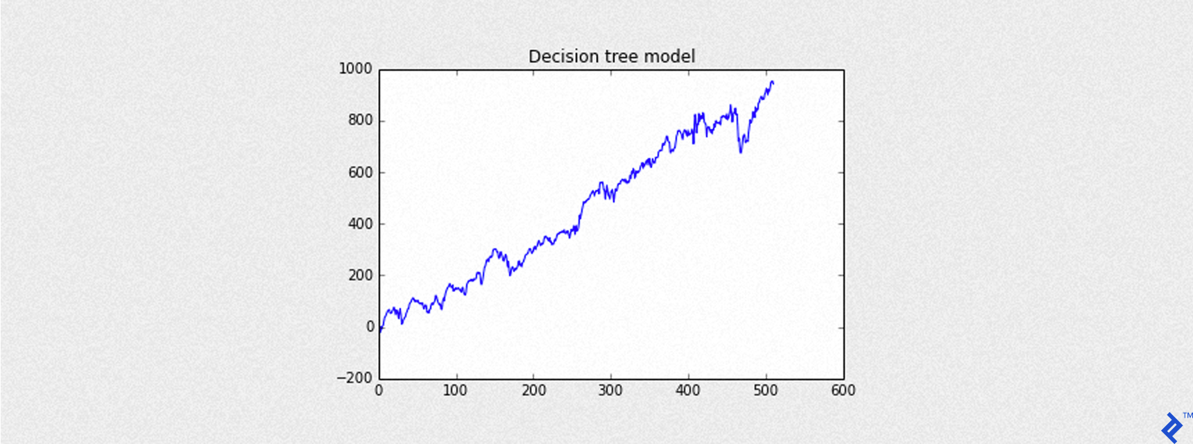
Mean of PnL is 1.843504
Sharpe is 1.972835
Round turns 511
Here, Sharpe is the Annual Sharpe ratio, an important indicator of the goodness of the trading model.
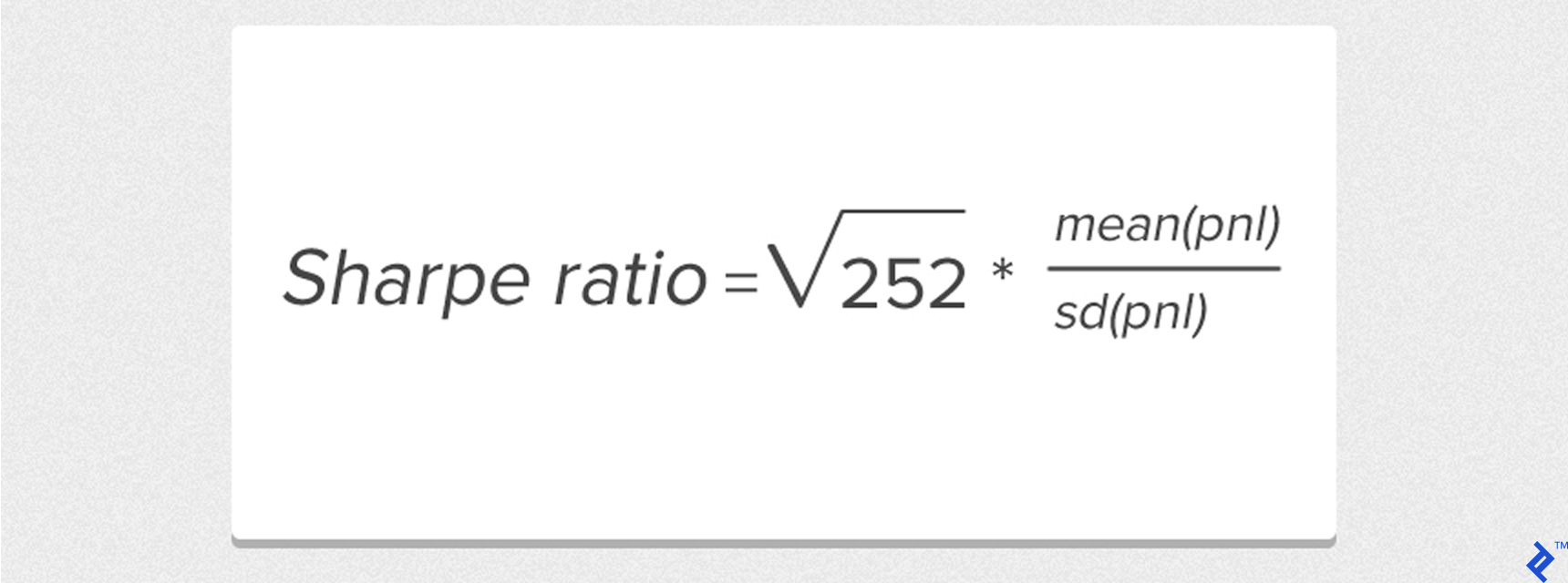
Considering trades expressed day by day whereas mean is the mean of the list of profit and loss, and sd is the standard deviation. For simplicity in the formula depicted above, I have considered a risk-free return equal to 0.
Some Basics About Trading
Trading the index requires buying an asset, which is directly derived from the index. Many brokers replicate the S&P 500 index with a derivative product called CFD (Contract for difference), which is an agreement between two parties to exchange the difference between the opening price and closing price of a contract.
Example: Buy 1 CFD S&P 500 at Open (value is 2000), sell it at Close of the day (value is 2020). The difference, hence the gain, is 20 points. If each point has a value of $25:
-
Gross Gain is
20 points x $25 = $500with 1 CFD contract.
Let’s say that the broker keeps a slippage of 0.6 points for its own revenue:
-
Net gain is
(20 - 0.6) points x $25 = $485.
Another important aspect to consider is to avoid significant losses within a trade. They may happen whenever the predicted outcome is +1 but the real outcome value is -1, so it is a false positive. In that case, the ending session turns out to be a Down day with a closing price lower than the opening, and we get a loss.
A stop loss order must be placed to protect against a maximum loss we would tolerate within a trade, and such an order is triggered whenever the price of the asset goes below a fixed value we have set before.
If we look at the time series downloaded from Yahoo Finance at the beginning of this article, every day has a Low price which is the lowest price reached during that day. If we set a stop level of -3 points far from the Opening price, and Low - Open = -5 the stop order will be triggered, and the opened position will be closed with a loss of -3 points instead of -5. This is a simple method to reduce the risk. The following code represents my helper function to simulate a trade with a stop level:
# This is a helper function to trade 1 bar (for example 1 day) with a Buy order at opening session
# and a Sell order at closing session. To protect against adverse movements of the price, a STOP order
# will limit the loss to the stop level (stop parameter must be a negative number)
# each bar must contains the following attributes:
# Open, High, Low, Close prices as well as gain = Close - Open and lo = Low - Open
def trade_with_stop(bar, slippage = 0, stop=None):
    """
    Given a bar, with a gain obtained by the closing price - opening price
    it applies a stop limit order to limit a negative loss
    If stop is equal to None, then it returns bar['gain']
    """
    bar['gain'] = bar['gain'] - slippage
    if stop<>None:
        real_stop = stop - slippage
        if bar['lo']<=stop:
            return real_stop
    # stop == None
    return bar['gain']
Trading Costs
Transaction costs are expenses incurred when buying or selling securities. Transaction costs include brokers’ commissions and spreads (the difference between the price the dealer paid for a security and the price the buyer pays), and they need to be considered if we want to backtest our strategy, similarly to a real scenario. Slippage in the trading of stocks often occurs when there is a change in spread. In this example and for the next ongoing simulations, trading costs are fixed as:
- Slippage = 0.6 points
- Commission = 1$ for each trade (one round turn will cost 2$)
Just to write some numbers, if our gross gain were 10 points, 1 point = $25, so $250 including trading costs, our net gain would be (10 - 0.6)*$25 - 2 = $233.
The following code shows a simulation of the previous trading strategy with a stop loss of -3 points. The blue curve is the curve of cumulative returns. The only costs accounted for are slippage (0.6 points), and the result is expressed in basis points (the same base unit of S&P 500 values downloaded from Yahoo Finance).
SLIPPAGE = 0.6
STOP = -3
trades = testing[testing['predictions'] == 1][('datetime', 'gain', 'ho', 'lo', 'open', 'close')]
trades['pnl'] = trades.apply(lambda x: trade_with_stop(x, slippage=SLIPPAGE, stop=STOP))
plot_equity_chart(trades['pnl'],'Decision tree model')
print("Slippage is %s, STOP level at %s" % (SLIPPAGE, STOP))
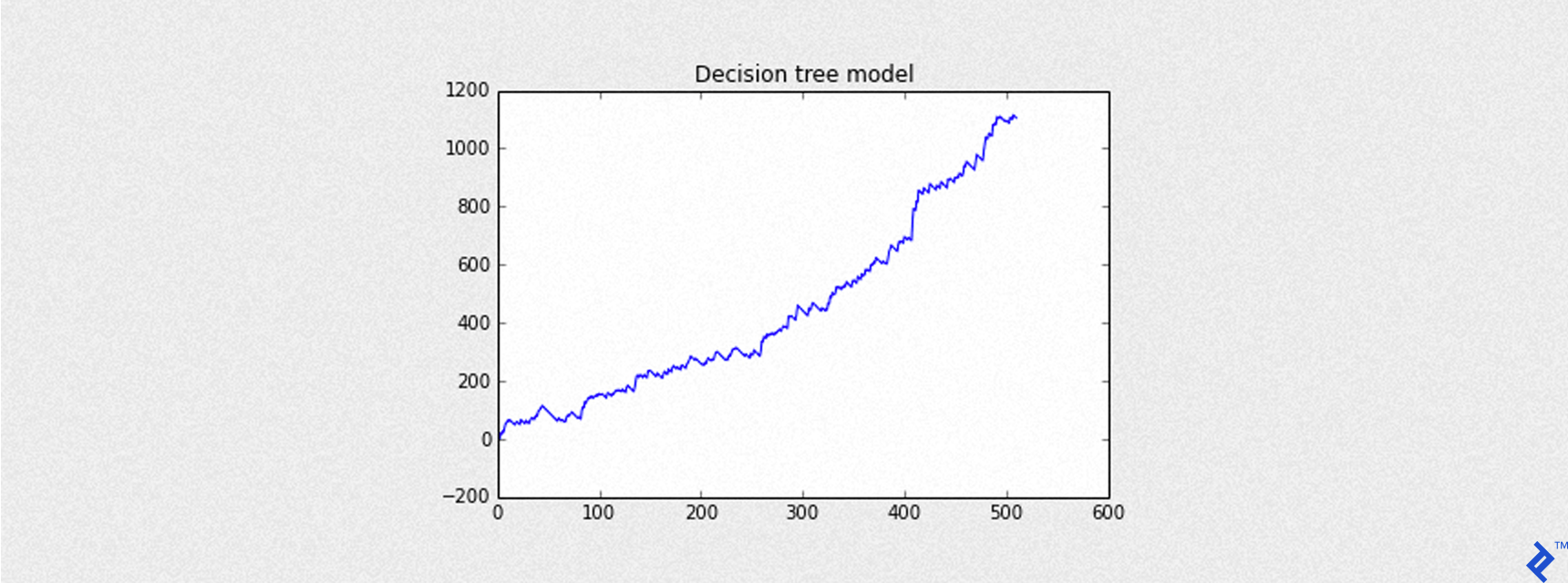
Mean of PnL is 2.162171
Sharpe is 3.502897
Round turns 511
Slippage is 0.6
STOP level at -3
The following code is used to make predictions in a slightly different way. Please pay attention to the predict method which is called with an additional parameter output_type = “probability”. This parameter is used to return probabilities of predicted values instead of their class prediction (+1 for a positively predicted outcome, -1 for a negatively predicted outcome). A probability greater than or equal to 0.5 is associated with a predicted value +1 and a probability value less than 0.5 is related to a predicted value of -1. The higher that probability is, the more chance we have to predict a real Up Day.
predictions_prob = decision_tree.predict(testing, output_type = 'probability')
# predictions_prob will contain probabilities instead of the predicted class (-1 or +1)
Now we backtest the model with a helper function called backtest_ml_model which calculates the series of cumulative returns including slippage and commissions, and plots their values. For brevity, without explaining thoroughly backtest_ml_model function, the important detail to highlight is that instead of filtering those days with a predicted outcome = 1 as we did in the previous example, now we filter those predictions_prob equal to or greater than a threshold = 0.5, as following:
trades = testing[predictions_prob>=0.5][('datetime', 'gain', 'ho', 'lo', 'open', 'close')]
Remember that Net gain of each trading day is: Net gain = (Gross gain - SLIPPAGE) * MULT - 2 * COMMISSION.
Another important metric used to evaluate the goodness of a trading strategy is the Maximum Drawdown. In general, it measures the largest single drop from peak to the bottom, in the value of an invested portfolio. In our case, it is the most significant drop from peak to bottom of the equity curve (we have just one asset in our portfolio, S&P 500). So given an SArray of profit and loss pnl, we calculate the drawdown as:
drawdown = pnl - pnl.cumulative_max()
max_drawdown = min(drawdown)
Inside the helper function backtest_summary is calculated:
- Maximum drawdown (in dollars) as shown above.
- Accuracy, with
Graphlab.evaluationmethod. - Precision, with
Graphlab.evaluationmethod. - Recall, with
Graphlab.evaluationmethod.
Putting it all together, the following example shows the equity curve representing cumulative returns of the model strategy, with all values expressed in dollars.
model = decision_tree
predictions_prob = model.predict(testing, output_type="probability")
THRESHOLD = 0.5
bt_1_1 = backtest_ml_model(testing, predictions_prob, target='outcome',
                           threshold=THRESHOLD, STOP=-3,
                           MULT=25, SLIPPAGE=0.6, COMMISSION=1, plot_title='DecisionTree')
backtest_summary(bt_1_1)
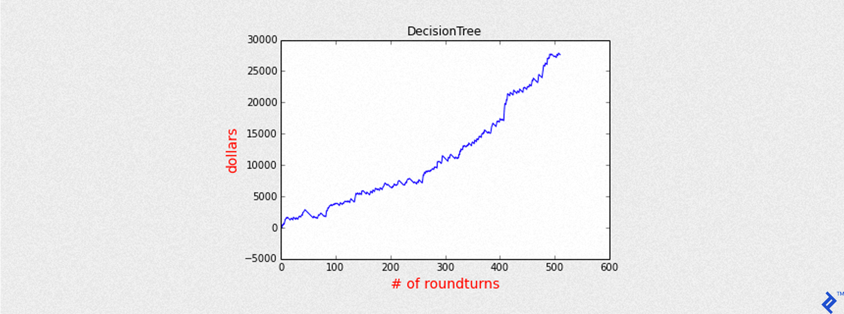
Mean of PnL is 54.054286
Sharpe is 3.502897
Round turns 511
Name: DecisionTree
Accuracy: 0.577373211964
Precision: 0.587084148728
Recall: 0.724637681159
Max Drawdown: -1769.00025
To increase the precision of forecasted values, instead of a standard probability of 0.5 (50 percent) we choose a higher threshold value, to be more confident that the model predicts an Up day.
THRESHOLD = 0.55
# it’s the minimum threshold to predict an Up day so hopefully a good day to trade
bt_1_2 = backtest_ml_model(testing, predictions_prob, target='outcome',
                           threshold=THRESHOLD, STOP=-3,
                           MULT=25, SLIPPAGE=0.6, COMMISSION=1, plot_title='DecisionTree')
backtest_summary(bt_1_2)
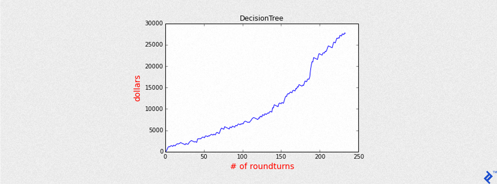
Mean of PnL is 118.244689
Sharpe is 6.523478
Round turns 234
Name: DecisionTree
Accuracy: 0.560468140442
Precision: 0.662393162393
Recall: 0.374396135266
Max Drawdown: -1769.00025
As we can see by the chart above, the equity curve is much better than before (Sharpe is 6.5 instead of 3.5), even with fewer round turns.
From this point on, we will consider all next models with a threshold higher than a standard value.
Training a Logistic Classifier
We can apply our research, as we did previously with the decision tree, into a Logistic Classifier model. GraphLab Create has the same interface with Logistic Classifier object, and we will call the create method to build our model with the same list of parameters. Moreover, we prefer to predict the probability vector instead of the predicted class vector (composed of +1 for a positive outcome, and -1 for a negative outcome), so we would have a threshold greater than 0.5 to achieve a better precision in our forecasting.
model = gl.logistic_classifier.create(training, target='outcome', features=l_features,
                                      validation_set=None, verbose=False)
predictions_prob = model.predict(testing, 'probability')
THRESHOLD = 0.6
bt_2_2 = backtest_ml_model(testing, predictions_prob, target='outcome',
                           threshold=THRESHOLD, STOP=-3, plot_title=model.name())
backtest_summary(bt_2_2)
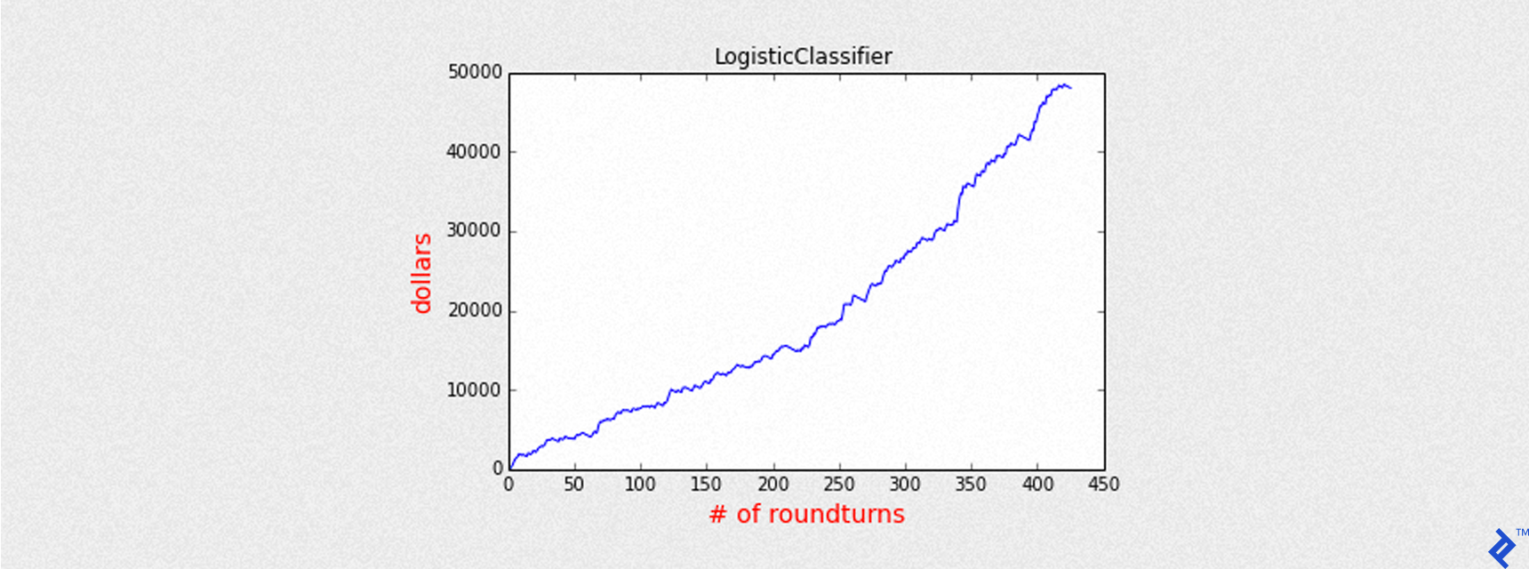
Mean of PnL is 112.704215
Sharpe is 6.447859
Round turns 426
Name: LogisticClassifier
Accuracy: 0.638491547464
Precision: 0.659624413146
Recall: 0.678743961353
Max Drawdown: -1769.00025
In this case, there is a summary very similar to Decision Tree. After all, both models are classifiers, they only predict a class of binary outcomes (+1, -1).
Training a Linear Regression Model
The main difference of this model is that it deals with continuous values instead of binary classes, as mentioned before. We don’t have to train the model with a target variable equal to +1 for Up days and -1 for Down days, our target must be a continuous variable. Since we want to predict a positive gain, or in other words a Closing price higher than the Opening price, now target must be the gain column of our training set. Also, the list of features must be composed of continuous values, such as the previous Open, Close, etc.
For brevity, I won’t go into the details of how to select the right features, as this is beyond the scope of this article, which is more inclined to show how we should apply different Machine Learning models over a data set. The list of parameters passed to the create method are:
-
training- it is a training set containing feature columns and a target column. -
target- it is the name of the column containing the target variable. -
validation_set- it is a dataset for monitoring the model’s generalization performance. In our case, we have novalidation_set. -
features- it is a list of column names of features used for training the model, for this model we will use another set respect to the Classifier models. -
verbose- iftrue, it will print progress information during training. -
max_iterations- it is the maximum number of allowed passes through the data. More passes over the data can result in a more accurately trained model.
model = gl.linear_regression.create(training, target='gain', features = l_lr_features,
                                   validation_set=None, verbose=False, max_iterations=100)
predictions = model.predict(testing)
# a linear regression model, predict continuous values, so we need to make an estimation of their
# probabilities of success and normalize all values in order to have a vector of probabilities
predictions_max, predictions_min = max(predictions), min(predictions)
predictions_prob = (predictions - predictions_min)/(predictions_max - predictions_min)
So far, we have predictions which is SArray of predicted gains, whereas predictions_prob is SArray with predictions values normalized. To have a good accuracy and a certain number of round turns, comparable with previous models, I’ve chosen a threshold value of 0.4. For a predictions_prob less than 0.4, the backtest_linear_model helper function will not open a trade because a Down day is expected. Otherwise, a trade will be opened.
THRESHOLD = 0.4
bt_3_2 = backtest_linear_model(testing, predictions_prob, target='gain', threshold=THRESHOLD,
                              STOP = -3, plot_title=model.name())
backtest_summary(bt_3_2)
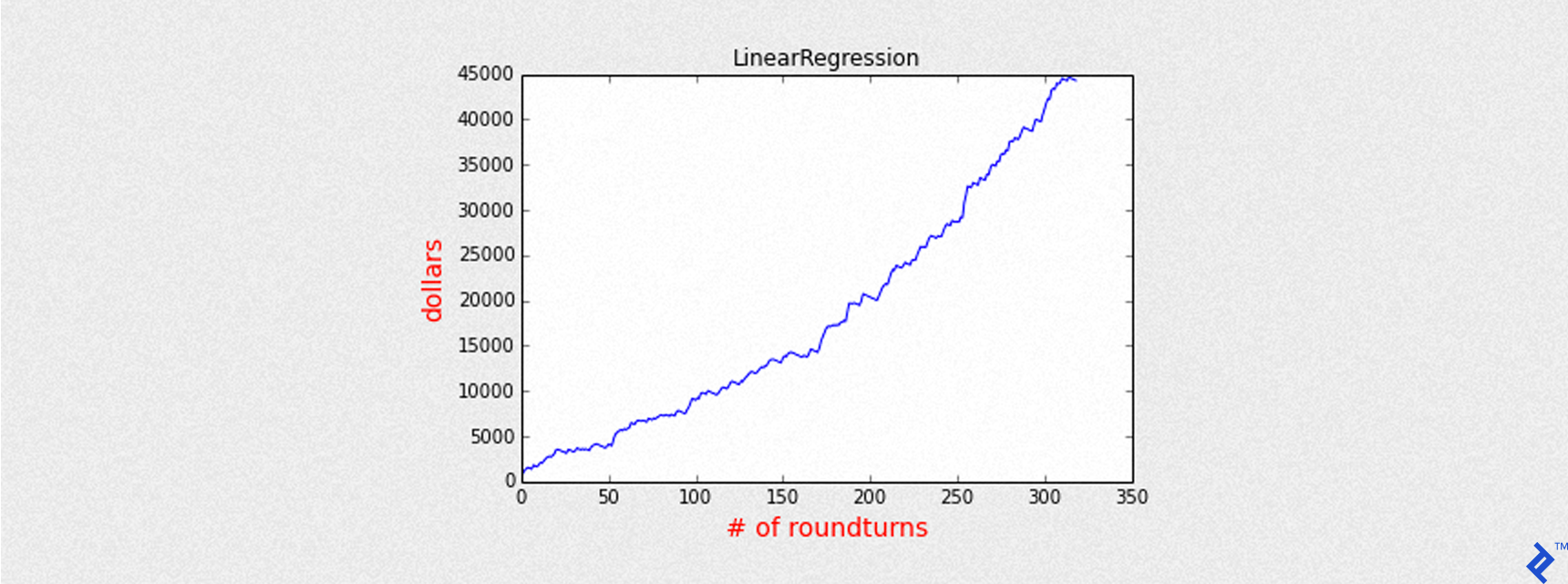
Mean of PnL is 138.868280
Sharpe is 7.650187
Round turns 319
Name: LinearRegression
Accuracy: 0.631989596879
Precision: 0.705329153605
Recall: 0.54347826087
Max Drawdown: -1769.00025
Training a Boosted Tree
As we previously did training a decision tree, now we are going to train a boosted tree classifier with the same parameters used for other classifier models. In addition, we set the number of max_iterations = 12 in order to increase the maximum number of iterations for boosting. Each iteration results in the creation of an extra tree. We also set a higher value of threshold than 0.5 to increase precision.
model = gl.boosted_trees_classifier.create(training, target='outcome', features=l_features,
                                           validation_set=None, max_iterations=12, verbose=False)
predictions_prob = model.predict(testing, 'probability')

THRESHOLD = 0.7
bt_4_2 = backtest_ml_model(testing, predictions_prob, target='outcome',
                           threshold=THRESHOLD, STOP=-3, plot_title=model.name())
backtest_summary(bt_4_2)
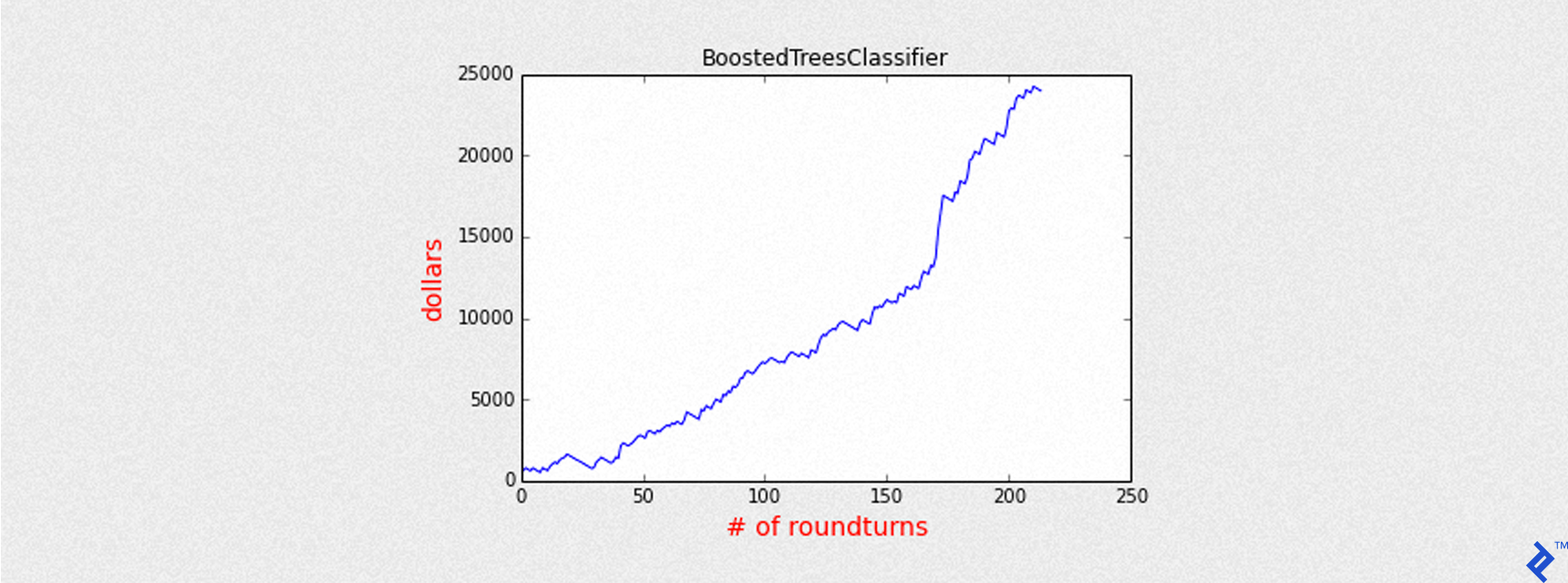
Mean of PnL is 112.002338
Sharpe is 6.341981
Round turns 214
Name: BoostedTreesClassifier
Accuracy: 0.563068920676
Precision: 0.682242990654
Recall: 0.352657004831
Max Drawdown: -1769.00025
Training a Random Forest
This is our last trained model, a Random Forest Classifier, composed by an ensemble of decision trees.
The maximum number of trees to use in the model is set to num_trees = 10, to avoid too much complexity and overfitting.
model = gl.random_forest_classifier.create(training, target='outcome', features=l_features,
                                      validation_set=None, verbose=False, num_trees = 10)
predictions_prob = model.predict(testing, 'probability')
THRESHOLD = 0.6
bt_5_2 = backtest_ml_model(testing, predictions_prob, target='outcome',
                           threshold=THRESHOLD, STOP=-3, plot_title=model.name())
backtest_summary(bt_5_2)

Mean of PnL is 114.786962
sharpe is 6.384243
Round turns 311
Name: RandomForestClassifier
Accuracy: 0.598179453836
Precision: 0.668810289389
Recall: 0.502415458937
Max Drawdown: -1769.00025
Collecting All the Models Together
Now we can join all the strategies together and see the overall result. It’s interesting to see the summary of all Machine Learning models, sorted by their precision.
| name | accuracy | precision | round turns | sharpe |
| LinearRegression | 0.63 | 0.71 | 319 | 7.65 |
| BoostedTreesClassifier | 0.56 | 0.68 | 214 | 6.34 |
| RandomForestClassifier | 0.60 | 0.67 | 311 | 6.38 |
| DecisionTree | 0.56 | 0.66 | 234 | 6.52 |
| LogisticClassifier | 0.64 | 0.66 | 426 | 6.45 |
If we collect all the profit and loss for each one of the previous models in the array pnl, the following chart depicts the equity curve obtained by the sum of each profit and loss, day by day.
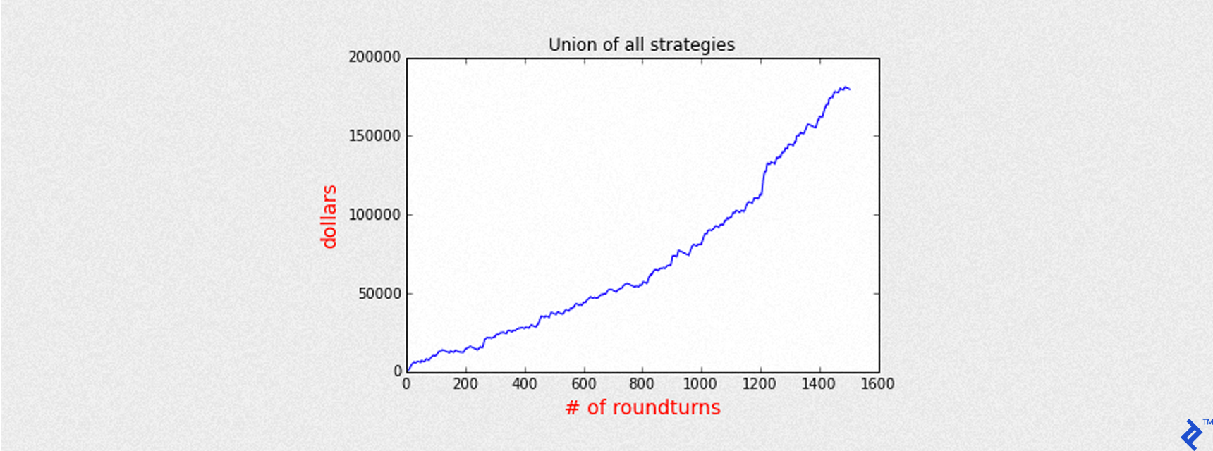
Mean of PnL is 119.446463
Sharpe is 6.685744
Round turns 1504
First trading day 2013-04-09
Last trading day 2016-04-22
Total return 179647
Just to give some numbers, with about 3 years of trading, all models have a total gain of about 180,000 dollars. The maximum exposition is 5 CFD contracts in the market, but to reduce the risk they all are closed at the end of each day, so overnight positions are not allowed.
Statistics of the Aggregation of All Models Together
Since each model can open a trade, but we added 5 concurrent models together, during the same day there could be from 1 contract up to 5 CFD contracts. If all models agree to open trades during the same day, there is a high chance to have an Up day predicted. Moreover, we can group by the number of models that open a trade at the same time during the opening session of the day. Then we evaluate precision as a function of the number of concurrent models.
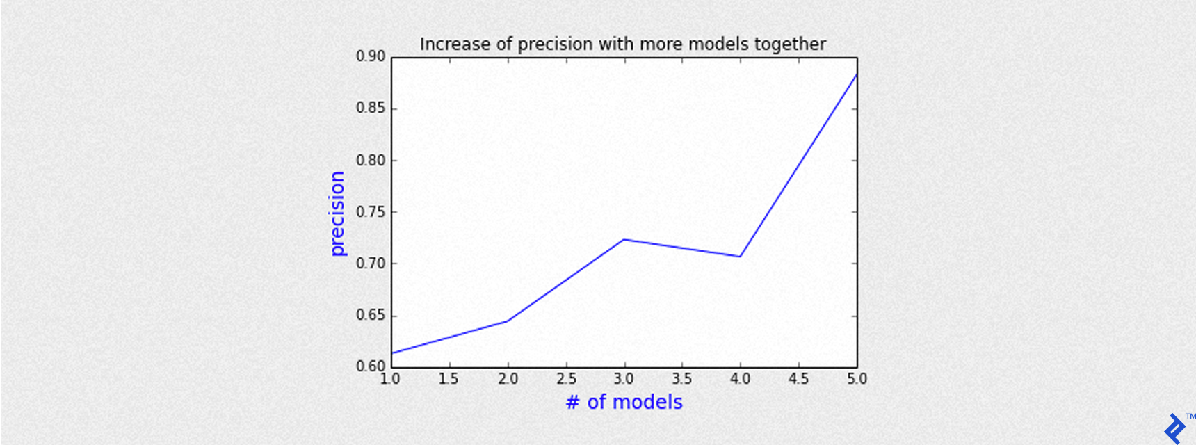
As we can see by the chart depicted above, the precision gets better as the number of models do agree to open a trade. The more models agree, the more precision we get. For instance, with 5 models triggered the same day, the chance to predict an Up day is greater than 85%.
Conclusion
Even in the financial world, Machine Learning is welcomed as a powerful instrument to learn from data and give us great forecasting tools. Each model shows different values of accuracy and precision, but in general, all models can be aggregated to achieve a better result than each one of them taken singularly. GraphLab Create is a great library, easy to use, scalable and able to manage Big Data very quickly. It implements different scientific and forecasting models, and there is a free license for students and Kaggle competitions.
Additional disclosure: This article has been prepared solely for information purposes, and is not an offer to buy or sell or a solicitation of an offer to buy or sell any security or instrument or to participate in any particular trading strategy. Examples presented on these sites are for educational purposes only. Past results are not necessarily indicative of future results.
Andrea Nalon
Venice, Metropolitan City of Venice, Italy
Member since March 23, 2016
About the author
With an MCE and extensive ML and quantitative analysis training, Andrea’s a data science experience covers R, Python, VBA, Excel, and SQL.
Expertise
PREVIOUSLY AT

