
Understanding Twitter Dynamics With R and Gephi: Text Analysis and Centrality
Centrality and text analysis allow users to get more out of their social network data. Here’s how you can leverage them using R and Gephi.

Centrality and text analysis allow users to get more out of their social network data. Here’s how you can leverage them using R and Gephi.

Juan is a developer, data scientist, and doctoral researcher at the University of Buenos Aires where he studies social networks, AI, and NLP. Juan has more than a decade of data science experience and has published papers at ML conferences, including SPIRE and ICCS.
Expertise
Previously At

This is the second installment in a three-part series on Twitter cluster analyses using R and Gephi. Part one laid the groundwork for the example we dive deeper into below; part three uses cluster analysis to draw conclusions from polarized posts about US politics.
Social Network Centrality
To achieve our goals, first we need to introduce the concept of centrality. In network science, centrality refers to nodes that have a strong influence on the network. Influence is an ambiguous concept; it can be understood in many ways. Is a node with many edges more influential than a node with fewer but more “important” edges? What constitutes an important edge on a social network?
To address these ambiguities, network scientists have developed many measures of centrality. Here, we discuss four commonly used measures, though many more are available.
Degree
The most common and intuitive measure is degree centrality. The idea behind degree centrality is simple: Measure the influence by the node’s degree. It can have variants if the graph is directed; in that case, you can measure the indegree and the outdegree—the first is known as the hub score and the second as the authority score.
In the first installment of this series, we used the undirected approach. This time, we focus on the indegree approach. This allows a more accurate analysis by emphasizing users who get retweeted by others over users who merely retweet frequently.
Eigenvector
The eigenvector measure builds upon degree centrality. The more that influential nodes point to a given node, the higher its score. We start with an adjacency matrix, where rows and columns represent nodes, and we use a 1 or 0 to indicate whether the corresponding nodes of a given row and column are connected. The main calculation estimates the matrix’s eigenvectors. The principal eigenvector will contain the centrality measures we want, where the position i will hold the centrality score of node i.
PageRank
PageRank is the variation of the eigenvector measure at the core of Google. The exact method Google uses is unknown, but the general idea is that each node starts with a score of 1, then distributes its score in equal parts to each of its edges. For example, if a node has three edges extending from it, it “sends” one third of its score through each edge. At the same time, the node is made more important by the edges that point to it. This results in a solvable system of N equations with N unknowns.
Betweenness
The fourth measure, betweenness, uses a very different approach. Here, a node is said to be influential if it is included in many short paths between other nodes. That is, it’s responsible for communicating with many other nodes, connecting “different worlds.”
For example, in social network analysis, these kinds of nodes could be understood as the types of people who help others find new jobs or make new connections—they are the doors to previously unknown social circles.
Which Should I Use?
The appropriate centrality measure depends on the goal of your analysis. Do you want to know which users are frequently singled out by others in terms of quantity? Degree centrality would likely be your best option. Or do you prefer a centrality measure that considers quality? In that case, eigenvector or PageRank will yield better results. If you want to know which users function most effectively as bridges between different communities, betweenness is your best option.
When using multiple similar measures, e.g., eigenvector and PageRank, you can estimate all of them and see if they yield equivalent rankings. If not, you can deepen your analysis of the differences or generate a new measure by combining their scores.
Another approach uses principal component analysis to estimate which measure gives you more information about the real influence of the nodes on your network.
Hands-on Centrality Calculation
Let’s see how we can calculate these measures using R and RStudio. (They can also be done with Gephi.)
First, we need to load all the libraries that we are going to use throughout this article:
library("plyr")
library(igraph)
library(tidyverse)
library(NLP)
library("tm")
library(RColorBrewer)
library(wordcloud)
library(topicmodels)
library(SnowballC)
library("textmineR")
Next, we will remove isolated nodes from the data we used before, as they are not useful to this analysis. Then, we will use the igraph functions betweenness, centr_eigen, page_rank, and degree to estimate the centrality measures. Finally, we will store the scores on the igraph object and on a data frame to see which users were the most central.
load("art1_tweets.RData")
Isolated = which(degree(net)==0)
net_clean = delete.vertices(net, Isolated)

cent<-data.frame(bet=betweenness(net_clean),eig=centr_eigen(net_clean)$vector,prank=(page_rank(net_clean)$vector),degr=degree(net_clean, mode="in"))
cent <- cbind(account = rownames(cent), cent)
Now we can check the 10 most central users by each measure:
| Degree | |
| Eigenvector | |
| PageRank | |
| Betweenness | |
The results:
| Degree | Eigenvector | PageRank | Betweenness | ||||
|---|---|---|---|---|---|---|---|
| ESPNFC | 5892 | PSG_inside | 1 | mundodabola | 0.037 | viewsdey | 77704 |
| TrollFootball | 5755 | CrewsMat19 | 0.51 | AleLiparoti | 0.026 | EdmundOris | 76425 |
| PSG_inside | 5194 | eh01195991 | 0.4 | PSG_inside | 0.017 | ba*****lla | 63799 |
| CrewsMat19 | 4344 | mohammad135680 | 0.37 | RoyNemer | 0.016 | FranciscoGaius | 63081 |
| brfootball | 4054 | ActuFoot_ | 0.34 | TrollFootball | 0.013 | Yemihazan | 62534 |
| PSG_espanol | 3616 | marttvall | 0.34 | ESPNFC | 0.01 | hashtag2weet | 61123 |
| IbaiOut | 3258 | ESPNFC | 0.3 | PSG_espanol | 0.007 | Angela_FCB | 60991 |
| ActuFoot_ | 3175 | brfootball | 0.25 | lnstantFoot | 0.007 | Zyyon_ | 57269 |
| FootyHumour | 2976 | SaylorMoonArmy | 0.22 | IbaiOut | 0.006 | CrewsMat19 | 53758 |
| mundodabola | 2778 | JohnsvillPat | 0.2 | 2010MisterChip | 0.006 | MdeenOlawale | 49572 |
We can see that the first three measures share a number of users, such as PSG_inside, ESPNFC, CrewsMat19, and TrollFootball. We can assume that they had a strong influence over the discussion. Betweenness has a different approach to measuring centrality and therefore doesn’t show as much overlap with the other techniques.
Note: Views expressed by the Twitter accounts mentioned in this article do not reflect those of Toptal or the author.
In the following images, you can see our original colored network graph with two user label overlays. In the first, the nodes are highlighted by their PageRank scores, and in the second, by their betweenness scores:


Gephi can be used to reproduce these images. You can estimate betweenness or PageRank scores using the Network Diameter button in the statistics panel. Then, you can show node names using attributes as demonstrated in the first installment in this series.
Text Analysis: R and LDA
We can also analyze social network discussions to identify what users have been talking about. There are multiple ways to approach this. We will do topic modeling through Latent Dirichlet Allocation (LDA), an unsupervised machine learning technique that allows us estimate which set of words tend to appear together. Then, through that set of words, we can infer the topic being discussed.
The first step is to sanitize the text. To do that, we define the following function:
# This function normalizes text by removing Twitter-related terms and noisy characters
sanitize_text <- function(text) {
  # Convert to ASCII to remove accented characters:
  text <- iconv(text, to = "ASCII", sub = " ")
  # Move to lower case and delete RT word (this is added by Twitter)
  text <- gsub("rt", " ", tolower(text))
  # Delete links and user names:
  text <- gsub("@\\w+", " ", gsub("http.+ |http.+$", " ", text))
  # Delete tabs and punctuation:
  text <- gsub("[ |\t]{2,}", " ", gsub("[[:punct:]]", " ", text))
  text <- gsub("amp", " ", text)  # Remove HTML special character
  # Delete leading and lagging blanks:
  text <- gsub("^ ", "", gsub(" $", "", text))
  text <- gsub(" +", " ", text) # Delete extra spaces
  return(text)
}
We also need to remove stop words, duplicates, and empty entries. Next, we have to convert our text to a document-term matrix to be processed by LDA.
In this dataset, we have users speaking in many languages (English, Spanish, French, etc.). LDA works best if we focus on a single language. We are going to apply it over the users of the biggest community detected in the first installment of this series, which is composed principally of accounts with English-speaking users.
# Detect communities:
my.com.fast <-cluster_louvain(as.undirected(simplify(net)))
largestCommunities <- order(sizes(my.com.fast), decreasing=TRUE)[1:3]
# Save the usernames of the biggest community:
community1 <- names(which(membership(my.com.fast) == largestCommunities[1]))

# Sanitize the text of the users of the biggest community:
text <- unique(sanitize_text(tweets.df[which(tweets.df$screen_name %in% community1),]$text))
text = text[text!=''] # Delete empty entries
stopwords_regex = paste(stopwords('es'), collapse = '\\b|\\b')
stopwords_regex = paste0('\\b', stopwords_regex, '\\b')
# Remove English stopwords:
text = stringr::str_replace_all(text, stopwords_regex, '')
# Create the document term matrix:
dtm <- CreateDtm(text,
                 doc_names = seq(1:length(text)),
                 ngram_window = c(1, 2))
Topic Counts and Coherence Scores
The main hyperparameter that we need to define in LDA is the number (k) of topics that we want to estimate. However, how can we know it beforehand? One common approach is to train LDA models over different k values and measure the coherence of each one. We’ll do this for k values from 3 up to 20, since values outside this range aren’t worth checking, in my experience:
tf <- TermDocFreq(dtm = dtm)
# Remove infrequent words:
tf_trimmed = tf$term[ tf$term_freq > 1 & tf$doc_freq < nrow(dtm) / 2 ]

# Create a folder to store trained models:
model_dir <- paste0("models_", digest::digest(tf_trimmed, algo = "sha1"))
if (!dir.exists(model_dir)) dir.create(model_dir)

# Define a function to infer LDA topics:
train_lda_model <- function(number_of_topics){
    filename = file.path(model_dir, paste0(number_of_topics, "_topics.rda"))
    # Check if the model already exists:
    if (!file.exists(filename)) {
        # To get exactly the same output on each run, use a constant seed:
        set.seed(12345)
        lda_model = FitLdaModel(dtm = dtm, k = number_of_topics, iterations = 500)
        lda_model$k = number_of_topics
        lda_model$coherence = CalcProbCoherence(phi = lda_model$phi, dtm = dtm, M = 5)
        save(lda_model, file = filename)
    } else {
        load(filename)
    }

    lda_model
}
# The number of topics that we are going to infer in each LDA training run:
topic_count = seq(3, 20, by = 1)
# Train through the TmParallelApply function
models = TmParallelApply(X = topic_count,
                         FUN = train_lda_model,
                         export = c("dtm", "model_dir"))
Next, we graph the coherence value of each:
coherence_by_topics_quantity = data.frame(
topic_number = sapply(models, function(model_instance) nrow(model_instance$phi)),
     score_coherence = sapply(models,
function(model_instance) mean(model_instance$coherence)),
     stringsAsFactors = FALSE)
ggplot(coherence_by_topics_quantity, aes(x = topic_number, y = score_coherence)) +
  geom_point() +
  geom_line(group = 1) +
  ggtitle("Coherence by Topic") + theme_minimal() +
  scale_x_continuous(breaks = seq(1,20,1)) + ylab("Coherence Score") + xlab("Number of topics")
A high coherence value shows a better segmentation of the text into topics:

We reach our peak coherence score with k = 13, so we’ll use the LDA model trained with 13 topics. Through the GetTopTerms function, we can see the 10 principal words for each topic and estimate the topic semantic through them:
best_model <- models[which.max(coherence_by_topics_quantity$score_coherence)][[ 1 ]]

# Most important terms by topic:
best_model$top_terms <- GetTopTerms(phi = best_model$phi, M = 20)
top10 <- as.data.frame(best_model$top_terms)
top10
The following table details the five most important topics detected and the 10 principal words that exemplify them:
| t_1 | t_2 | t_3 | t_4 | t_5 | |
|---|---|---|---|---|---|
| 1 | messi | messi | messi | messi | messi |
| 2 | lionel | league | est | psg | |
| 3 | lionel_messi | post | win | il | leo |
| 4 | psg | million | goals | au | leo_messi |
| 5 | madrid | likes | ch | pour | ahora |
| 6 | real | spo | ions | pas | compa |
| 7 | barcelona | goat | ch_ions | avec | va |
| 8 | paris | psg | ucl | du | ser |
| 9 | real_madrid | bar | ballon | qui | jugador |
| 10 | mbapp | bigger | world | je | mejor |
Although most users in this community are English speakers, there are still a number of French and Spanish speakers (t_4 and t_5 in the table). We can infer that the first topic relates to Messi’s previous team (FC Barcelona), the second topic is about Messi’s post on Instagram, and the third topic focuses on Messi’s achievements.
Now that we have the topics, we can predict which of them was the most discussed. To do that, we will first concatenate tweets by users (again, from the largest community):
tweets.df.com1 = tweets.df[which(tweets.df$screen_name %in% community1),]
users_text <- ddply(tweets.df.com1,
                    ~screen_name,
                    summarise,
                    text = paste(text, collapse = " "))
Then, we sanitize text as before and create the DTM. After that, we call the predict function using our LDA model and the DTM as arguments. Also, we set the method to Gibbs to improve computing time because we have a lot of text to analyze:
users_text$text <- sanitize_text(users_text$text) # Get rid of duplicates
stopwords_regex = paste(stopwords('en'), collapse = '\\b|\\b')
stopwords_regex = paste0('\\b', stopwords_regex, '\\b')
users_text$text = stringr::str_replace_all(users_text$text, stopwords_regex, '')

dtm.users.com1 <- CreateDtm(users_text$text,
                 doc_names = users_text$screen_name,
                 ngram_window = c(1, 2))
com1.users.topics = predict(best_model, dtm.users.com1, method="gibbs", iterations=100)
Now, in the com1.users.topics data frame, we see how much each user talked about each topic:
| Account | t_1 | t_2 | t_3 | t_4 | t_5 | […] |
|---|---|---|---|---|---|---|
| ___99th | 0.02716049 | 0.86666666 | 0.00246913 | 0.00246913 | 0.00246913 | |
| Boss__ | 0.05185185 | 0.84197530 | 0.00246913 | 0.00246913 | 0.00246913 | |
| Memphis | 0.00327868 | 0.00327868 | 0.03606557 | 0.00327868 | 0.00327868 | |
| ___Alex1 | 0.00952380 | 0.00952380 | 0.00952380 | 0.00952380 | 0.00952380 | |
| […] |
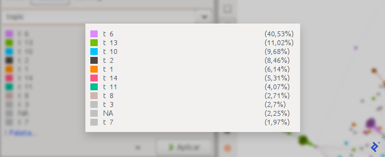
Finally, with this information, we can create a new attribute on the node graph to define which topic was most talked about by which user. Then we can create a new GML file to visualize it in Gephi:
# Get the subgraph of the first community:
net.com1 = induced_subgraph(net,community1)
# Estimate the topic with the max score for each user:
com1.users.maxtopic = cbind(users_text$screen_name,
                            colnames(com1.users.topics)[apply(com1.users.topics,
                                                              1,
                                                              which.max)])
# Order the users topic data frame by the users' order in the graph:
com1.users.maxtopic = com1.users.maxtopic[match(V(net.com1)$name,
                                          com1.users.maxtopic[,1]),]
# Create a new attr of the graph by the topic most discussed by each user:
V(net.com1)$topic = com1.users.maxtopic[,2]
# Create a new graph:
write_graph(simplify(net.com1),  "messi_graph_topics.gml", format = "gml")

Inferring Important Topics and Applying Social Network Centrality
In the first installment of this series, we learned how to obtain data from Twitter, create the interaction graph, plot it through Gephi, and detect communities and important users. In this installment, we expanded upon this analysis by demonstrating the use of additional criteria to detect influential users. We also demonstrated how to detect and infer what the users were talking about and plot that in the network.
In our next article, we will continue to deepen this analysis by showing how users can explore clustered social media data.
Also in This Series:
Further Reading on the Toptal Blog:
Understanding the basics
Centrality is a measure that, in the context of social network analysis, can help us detect influential users on the network.
Degree centrality measures the influence of a user by the number of edges that they have.
Eigenvector centrality measures the influence of a user by the number and quality of edges that they have.
Betweenness centrality measures the influence of a user by how many users connect through them.
RStudio is an integrated development environment (IDE) for programming in R.
R is a powerful programming language designed to perform text analysis. It has many libraries for classic text analysis tasks, such as sentiment analysis for topic modeling.
Juan Manuel Ortiz de Zarate
Buenos Aires, Argentina
Member since November 6, 2019
About the author
Juan is a developer, data scientist, and doctoral researcher at the University of Buenos Aires where he studies social networks, AI, and NLP. Juan has more than a decade of data science experience and has published papers at ML conferences, including SPIRE and ICCS.
Expertise
PREVIOUSLY AT