Optimized Successive Mean Quantization Transform
Image processing algorithms are often very resource intensive due to fact that they process pixels on an image one at a time and often requires multiple passes. Successive Mean Quantization Transform (SMQT) is one such resource intensive algorithm that can process images taken in low-light conditions and reveal details from dark regions of the image.
In this article, Toptal engineer Daniel Angel Munoz Trejo gives us some insight into how the SMQT algorithm works and walks us through a clever optimization technique to make the algorithm a viable option for handheld devices.

Daniel has created high-performance applications in C++ for large companies such as Dreamworks. He also excels with C and ASM (x86).
PREVIOUSLY AT

Successive Mean Quantization Transform (SMQT) algorithm is a non-linear transformation that reveals the organization or structure of the data and removes properties such as gain and bias. In a paper titled The Successive Mean Quantization Transform, SMQT is “applied in speech processing and image processing”. The algorithm when applied to images “can be seen as a progressive focus on the details in an image”.

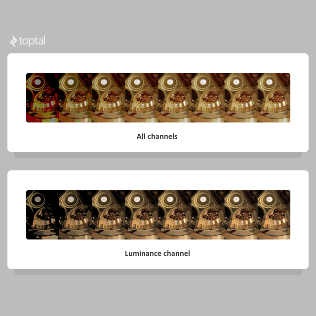
According to another paper titled SMQT-based Tone Mapping Operators for High Dynamic Range Images, it will yield an “image with enhanced details”. The paper describes two techniques of applying this transformation to an image.
-
Apply SMQT on luminance of each pixel - it describes the formula to obtain the luminance from the RGB of each pixel.
-
Apply SMQT on each channel of RGB separately - for channels R, G, and B individually.
The following picture shows the result of the two techniques:
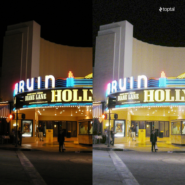
By applying the second technique to a picture of Bruin Theatre at night, we can see how the algorithm progressively zooms on the details of the image and reveals details that are originally hidden by the darkness:
In this article, we will take a closer look at how this algorithm works, and explore a simple optimization that allows the algorithm to be much more performant in practical image processing applications.
The SMQT Algorithm
In the original paper, the algorithm is described in an abstract manner. To better understand SMQT, we will walk through some simple examples.
Suppose we have the following vector (you can think of it like an array):
| 32 | 48 | 60 | 64 | 59 | 47 | 31 | 15 | 4 | 0 | 5 | 18 |
In case of a color image, we can think of it as three separate vectors, each representing a particular color channel (RGB), and each element of the vector representing the intensity of the corresponding pixel.
The steps involved in applying the SMQT algorithm are:
-
Calculate the mean of the vector, which in this case is 29.58.
-
Split the vector in two, leaving the numbers that are less or equal than 29.58 in the left half, and the numbers that are greater in the right half:
15 4 0 5 18 32 48 60 64 59 47 31 0 0 0 0 0 1 1 1 1 1 1 1 The second row is the code we will create for each value. The values lower than or equal to 29.58 get a 0 in its code, and the numbers greater than 29.58 get a 1 (this is binary).
-
Now both resulting vectors are split individually, in a recursive way, following the same rule. In our example the mean of the first vector is (15 + 4 + 0 + 5 + 18) / 5 = 8.4, and the mean of the second vector is (32 + 48 + 60 + 64 + 59 + 47 + 31) / 7 = 48.7. Each of those two vectors is further split into two more vectors, and a second bit of code is added to each depending on its comparison with the mean. This is the result:
4 0 5 15 18 32 47 31 48 60 64 59 00 00 00 01 01 10 10 10 11 11 11 11 Note that a 0 was again appended for numbers lower than or equal to the mean (for each vector) and a 1 for numbers greater than the mean.
-
This algorithm is repeated recursively:
0 4 5 15 18 32 31 47 48 60 64 59 000 001 001 010 011 100 100 101 110 111 111 111 0 4 5 15 18 31 32 47 48 60 59 64 0000 0010 0011 0100 0110 1000 1001 1010 1100 1110 1110 1111 0 4 5 15 18 31 32 47 48 59 60 64 00000 00100 00110 01000 01100 10000 10010 10100 11000 11100 11101 11110 At this point every vector has only one element. So for every successive step a 0 will be appended, since the number will always be equal to itself (the condition for a 0 is that the number must be less than or equal to the mean, which is itself).
So far we have a quantization level of L=5. If we were going to use L=8, we must append three 0s to each code. The result of converting each code from binary to integer (for L=8) would be:
| 0 | 4 | 5 | 15 | 18 | 31 | 32 | 47 | 48 | 59 | 60 | 64 |
| 0 | 32 | 48 | 64 | 96 | 128 | 144 | 160 | 192 | 224 | 232 | 240 |
The final vector is sorted in increasing order. To obtain the output vector, we must substitute the original value of the input vector by its code.
| 32 | 48 | 60 | 64 | 59 | 47 | 31 | 15 | 4 | 0 | 5 | 18 |
| 144 | 192 | 232 | 240 | 224 | 160 | 128 | 64 | 32 | 0 | 48 | 96 |
Notice that in the resulting vector:
- The gain was removed. The original one had a low gain, with its range going from 0 to 64. Now its gain goes from 0 to 240, which is almost the entire 8 bit range. It is said that the gain is removed because it doesn’t matter if we multiply all the elements of the original vector by a number, such as 2, or if we divide all by 2, the output vector would be about the same. Its range would be about the entire range of the destination vector (8 bits for L=8). If we multiply the input vector by two, the output vector will actually be the same, because in each step the same numbers that were below or above the mean will continue to be below or above it, and we will add the same 0s or 1s to the output. Only if we divide it would the result be about the same, and not exactly the same, because odd numbers like 15 will have to be rounded and the calculations may vary then. We went from a dark image to an image with its pixels ranging from dark colors (0) to lighter colors (240), using the entire range.
- The bias is removed, although we can’t quite observe it in this example. This is because we don’t have a bias since our lowest value is 0. If we actually had a bias, it’d have been removed. If we take any number ‘K’ and add it to each element of the input vector, the calculation of the numbers above and below the mean in each step will not vary. The output will still be the same. This would also make images that are too bright to become images that range from dark to light colors.
- We have an image with enhanced details. Note how for each recursive step we take we are actually zooming into the details, and constructing the output by revealing those details as much as possible. And since we will apply this technique to each RGB channel, we will reveal as many details as possible, although losing information about the original tones of each color.
Given an image like a vector of RGB pixels, with each point being 8 bits for R, 8 for G, and 8 for B; we can extract three vectors from it, one for each color, and apply the algorithm to each vector. Then we form the RGB vector again from those three output vectors and we have the SMQT processed image, as done with the one of the Bruin Theatre.
Complexity
The algorithm requires that for each level of quantization (L), N elements must be inspected in a first pass to find the mean for each vector, and then in a second pass, each of those N elements must be compared to the corresponding mean in order to split each vector in turn. Finally, N elements must be substituted by their codes. Therefore the algorithm’s complexity is O((L*2*N) + N) = O((2*L + 1)*N), which is O(L*N).
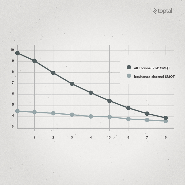
The graph extracted from the paper is consistent with the O(L*N) complexity. The lower the L, the faster the processing in an approximately linear way (greater number of frames per second). In order to improve processing speed, the paper suggests lowering values of L: “selecting a level L lower can be a direct way to reduce processing speed but with reduced image quality”.
Improvement
Here we will find a way to improve speed without reducing image quality. we will analyze the transformation process and find a faster algorithm. In order to get a more complete perspective on this, let’s see an example with repeated numbers:
| 16 | 25 | 31 | 31 | 25 | 16 | 7 | 1 | 1 | 7 |
| 16 | 16 | 7 | 1 | 1 | 7 | 25 | 31 | 31 | 25 |
| 0 | 0 | 0 | 0 | 0 | 0 | 1 | 1 | 1 | 1 |
| 7 | 1 | 1 | 7 | 16 | 16 | 25 | 25 | 31 | 31 |
| 00 | 00 | 00 | 00 | 01 | 01 | 10 | 10 | 11 | 11 |
| 1 | 1 | 7 | 7 | 16 | 16 | 25 | 25 | 31 | 31 |
| 000 | 000 | 001 | 001 | 010 | 010 | 100 | 100 | 110 | 110 |
The vectors cannot be split any more, and zeros must be appended until we get to the desired L.
For the sake of simplicity, let’s suppose that the input can go from 0 to 31, and the output from 0 to 7 (L=3), as it can be seen in the example.
Note that computing the mean of the first vector (16 + 25 + 31 + 31 + 25 + 16 + 7 + 1 + 1 + 7) / 10 = 16 gives the same result as computing the mean of the entire last vector, since it’s just the same vector with the elements in a different order: (1 + 1 + 7 + 7 + 16 + 16 + 25 + 25 + 31 + 31) / 10 = 16.
In the second step we must compute each vector recursively. So we compute the mean of the grayed inputs, which are the first 6 elements ((16 + 16 + 7 + 1 + 1 + 7) / 6 = 8), and the mean of the blank input, which are the last 4 elements ((25 + 31 + 31 + 25) / 4 = 28):
| 16 | 16 | 7 | 1 | 1 | 7 | 25 | 31 | 31 | 25 |
Note again that if we use the last vector, the one that is completely ordered, the results are the same. For the first 6 elements we have: ((1 + 1 + 7 + 7 + 16 + 16) / 6 = 8), and for the last 4 elements: ((25 + 25 + 31 + 31) / 4 = 28). Since it’s just an addition the order of the summands does not matter.
| 1 | 1 | 7 | 7 | 16 | 16 | 25 | 25 | 31 | 31 |
The same applies for the next step:
| 7 | 1 | 1 | 7 | 16 | 16 | 25 | 25 | 31 | 31 |
The calculations are the same as with the last vector: ((7 + 1 + 1 + 7) / 4 = 4) will be equal to ((1 + 1 + 7 + 7) / 4 = 4).
And the same will apply for the rest of the vectors and steps.
The calculation of the mean is just the sum of the values of the elements in the interval, divided by the number of elements in the interval. This means that we can precompute all those values and avoid repeating this calculation L times.
Let’s see the steps to apply what we will call FastSMQT algorithm to our example:
-
Create a table with 32 columns and 3 rows as you can see below. The first row in the table represents the index of the table (0 to 31) and is not necessary to be included when coding the table. But it’s explicitly shown to make the example easier to follow.
-
Iterate the N elements once counting the frequency of each value. In our example, elements 1, 7, 16, 25 and 31 all have a frequency of 2. All the other elements have a frequency of 0. This step has a complexity of O(N).
-
Now that the frequency vector is filled, we need to iterate that vector (the frequencies vector, not the input vector). We don’t iterate N elements anymore, but R (R being in the range: 2^L), which in this case is 32 (0 to 31). When processing pixels, N can be many millions (megapixels), but R is usually 256 (one vector for each color). In our example it’s 32. we will fill the following two rows of the table at the same time. The first of those rows (the second of the table) will have the sum of the frequencies so far. The second (the third of the table) will have the sum of the value of all elements that appeared so far.
In our example, when we get to 1, we put a 2 in the second row of the table because two 1s have appeared so far. And we also put a 2 in the third row of the table, because 1 + 1 = 2. We continue writing those two values on each of the next positions until we get to 7. Since number 7 appears twice, we add 2 to the accumulator of the second row, because now 4 numbers appeared so far (1, 1, 7, 7). And we add 7 + 7 = 14 to the third row, resulting in 2 + 14 = 16, because 1 + 1 + 7 + 7 = 16. We continue with this algorithm until we finish iterating those elements. The complexity of this step is O(2^L), which in our case is O(32), and when working with RGB pixels it’s O(256).
i 0 1 2 ... 6 7 8 ... 15 16 17 ... 24 25 26 ... 30 31 n 0 2 0 ... 0 2 0 ... 0 2 0 ... 0 2 0 ... 0 2 n-cumulative 0 2 2 ... 2 4 4 ... 4 6 6 ... 6 8 8 ... 8 10 sum 0 2 2 ... 2 16 16 ... 16 48 48 ... 48 98 98 ... 98 160 -
The next step is to remove from the table the columns with elements that have a frequency of 0, and to see the example clearer we will also remove the second row since it’s not relevant anymore, as you will see.
i 1 7 16 25 31 n 2 4 6 8 10 sum 2 16 48 98 160 -
Remember that we could use the last (completely ordered) vector to do the calculations for each step and the results will still be the same. Note that here, in this table, we have the last vector with all the pre-calculations already made.
We basically need to do the SMQT algorithm on this small vector, but unlike doing it on the original vector that we started with, this one will be much more easier.
First we need to calculate the mean of all the samples. We can find it easily by: sum[31] / n[31] = 160 / 10 = 16. So we split the table in two vectors, and start writing the binary code for each:
i 1 7 16 25 31 n 2 4 6 8 10 sum 2 16 48 98 160 code 0 0 0 1 1 Now we split each vector again. The mean of the first vector is: sum[16] / n[16] = 48 / 6 = 8. And the mean of the second vector is: (sum[31] – sum[16]) / (n[31] – n[16]) = (160 – 48) / (10 – 6) = 112 / 4 = 28.
i 1 7 16 25 31 n 2 4 6 8 10 sum 2 16 48 98 160 code 00 00 01 10 11 There is only one vector left to split. The mean is: sum[7] / n[7] = 16 / 4 = 4.
i 1 7 16 25 31 n 2 4 6 8 10 sum 2 16 48 98 160 code 000 001 010 100 110 As you can see, the code for each element is the same if we had followed the original algorithm. And we did the SMQT on a much smaller vector than the one with N elements and we also have pre calculated all the values we need in order to find the mean, so it’s straightforward and fast to compute the resulting vector.
The complexity of this step is O(L*(2^L)), which for an L=8, and in practical image processing needs, it’s O(8*(256)) = O(2048) = constant.
-
The final step is to iterate N elements once again replacing the element by its code for each element: element[i] = code[i]. The complexity is O(N). The complexity of FastSMQT is O(N) + O(2^L) + O(L*(2^L)) + O(N) = O(2*N) + O((L + 1)*(2^L)) = O(N + L*(2^L)) .
Parallelism
Both algorithms can be parallelized, although it’s more efficient to run one algorithm per core instead if multiple vectors must be transformed. For example, when processing images we can process each RGB channel in a different core instead of parallelizing each of those three calculations.
To parallelize SMQT algorithm, when we divide a vector in two, we can process each sub-vector in a new core if a core is available (actually one sub vector in current core and the other in a new core). This can be done recursively until we reach the total number of available cores. The replacements of values by codes can also be done in a parallel for.
FastSMQT algorithm can also be parallelized. In the first step, the input vector must be divided into the number of available cores (C). One vector of frequency count must be created for each of those parts, and be filled in parallel. Then we add the values of those vectors into one resulting vector of frequencies. The next step that can be parallelized is the last one, when we are substituting the values by their codes. This can be done in a parallel for.
Complexity Comparison
The total complexity of original SMQT algorithm is O((2*L + 1)*N), which is O(L*N).
The complexity of FastSMQT is O(N) + O(2^L) + O(L*(2^L)) + O(N) = O(2*N) + O((L + 1)*(2^L)) = O(N + L*(2^L)).
Given a fixed L, the complexity becomes just O(N) for both. But the constant that multiplies N are much smaller for FastSMQT, and it makes a big difference in processing time as we will see.
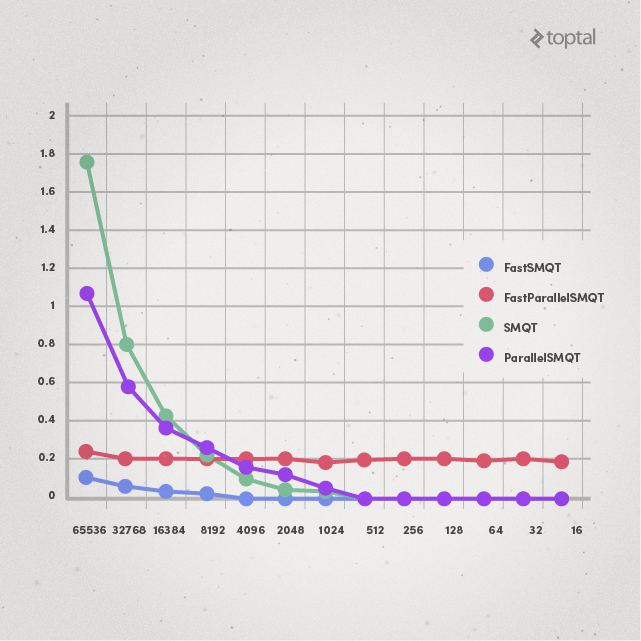
The following graph compares the performance of both SMQT and FastSMQT algorithms for L=8, which is the case for image processing. The graph shows the time (in milliseconds) that it takes to process N elements. Note that the complexity (with constants) of SMQT for L=8 is O(17*N), while for FastSMQT is O(2*N + 2304).

The bigger the N, the longer it takes for SMQT to process the image. For FastSMQT on the other hand, the growth is much slower.
For even bigger values of N, the difference in performance is much more apparent:

Here SMQT takes up to multiple seconds of time to process certain images, while FastSMQT still lies within the “few milliseconds” zone.
Even with multiple cores (two, in this case), FastSMQT is clearly still superior to just SMQT:
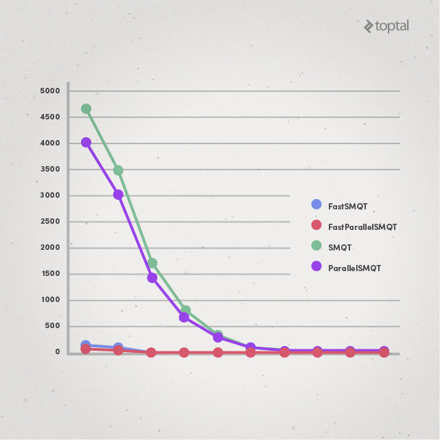
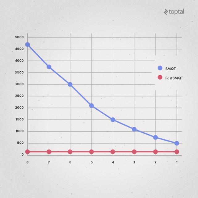
FastSMQT isn’t dependent on L. SMQT, on the other hand, is linearly dependent on the value of L. For example, with N = 67108864, the runtime of SMQT increases with increasing value of L, while FastSMQT doesn’t:
Conclusion
Not all optimization techniques are applicable for all algorithms, and the key to improving an algorithm’s performance is often hidden within some insight of how the algorithm works. This FastSMQT algorithm takes advantage of the possibilities of precalculating values and the nature of mean calculations. As a result it allows faster processing than the original SMQT. The speed is not affected by the increment of L, although L cannot be much greater than the usual 8 because memory usage is 2^L, which for 8 is an acceptable 256 (number of columns in our frequency table), but the performance gain has obvious practical benefits.
This improvement in speed allowed MiddleMatter to implement the algorithm in an iOS application (and an Android application) that improves pictures and videos captured in low light conditions. With this improvement, it was possible to perform video processing in application, which would otherwise be too slow for iOS devices.
The C++ code for SMQT and FastSMQT algorithms are available on GitHub.
Daniel Munoz
Seattle, WA, United States
Member since December 5, 2013
About the author
Daniel has created high-performance applications in C++ for large companies such as Dreamworks. He also excels with C and ASM (x86).
PREVIOUSLY AT